## Partition Plot: Input Space Partitioning ### Overview The image is a partition plot visualizing the partitioning of an input space. The space is divided into rectangular regions of varying sizes, with a higher density of smaller regions concentrated in specific areas. The plot is bounded by axes labeled x1 and x2, both ranging from -5 to 5. ### Components/Axes * **Title:** "Partition of input space" * **X-axis:** "-5 < x1 < 5" with tick marks at -5, 0, and 5. * **Y-axis:** "-5 < x2 < 5" with tick marks at -5, -4, -3, -2, -1, 0, 1, 2, 3, 4, and 5. * **Partitioning:** The space is divided into rectangular cells, with cell size varying across the space. The cells are defined by blue lines. ### Detailed Analysis The plot shows a rectangular area divided into smaller rectangles. The density of these smaller rectangles is not uniform. There are regions where the rectangles are very small and densely packed, and other regions where the rectangles are larger and more sparse. * **Dense Regions:** There are three primary regions of high density: * A region centered approximately at (-2, -2). * A region centered approximately at (-2, 3). * A region centered approximately at (1, 1). * **Sparse Regions:** The regions outside of the dense areas have larger rectangles. The largest rectangles are found in the corners of the plot. ### Key Observations * The partitioning is adaptive, with finer partitions in regions of interest. * The regions of interest appear to be clustered around specific coordinates. * The plot suggests a non-uniform distribution or function being approximated. ### Interpretation The plot likely represents the result of a space-partitioning algorithm, such as a decision tree or a k-d tree. The dense regions indicate areas where the algorithm has identified significant variations or decision boundaries, requiring finer resolution. The sparse regions indicate areas where the algorithm has determined that coarser resolution is sufficient. The plot visualizes how the input space is divided based on some underlying data or function. The concentration of smaller rectangles suggests that the function being approximated has more complexity in those regions.

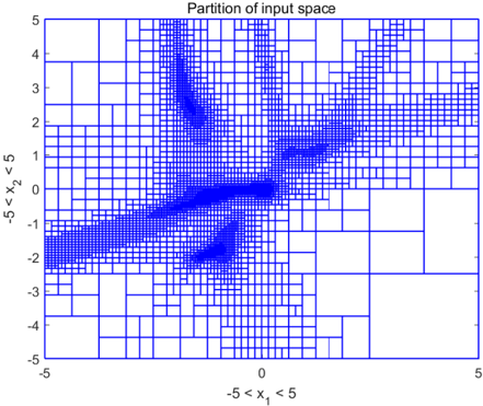
## Chart Type: Adaptive Spatial Partitioning Grid ### Overview This image displays a two-dimensional input space partitioned by an adaptive grid, likely a quadtree structure. The grid cells vary significantly in size, with smaller, higher-resolution cells concentrated in specific regions, which are also filled with a solid blue color. These blue-filled regions represent areas of interest or specific characteristics within the input space, while the white areas are covered by larger, lower-resolution cells. ### Components/Axes * **Title**: "Partition of input space" is centered at the top of the plot. * **X-axis**: * **Label**: "-5 < x₁ < 5" is centered below the x-axis. * **Range**: The axis spans from -5 to 5. * **Major Tick Markers**: -5, -4, -3, -2, -1, 0, 1, 2, 3, 4, 5. * **Y-axis**: * **Label**: "-5 < x₂ < 5" is positioned vertically along the left side of the y-axis. * **Range**: The axis spans from -5 to 5. * **Major Tick Markers**: -5, -4, -3, -2, -1, 0, 1, 2, 3, 4, 5. * **Grid Lines**: The entire input space is divided by a network of blue grid lines forming rectangular cells. * **Legend**: There is no explicit legend. The blue color is used for both the grid lines and to fill specific regions within the grid. ### Detailed Analysis The plot shows a 10x10 unit square input space, defined by x₁ from -5 to 5 and x₂ from -5 to 5. This space is adaptively partitioned into rectangular cells. **Grid Structure**: The grid is non-uniform. In areas where the input space is "empty" (white background), the cells are generally large, indicating a coarse partitioning. Conversely, in regions that are filled with blue, the cells become significantly smaller, indicating a finer, higher-resolution partitioning. This adaptive refinement is a key characteristic of quadtree-like structures. **Blue Shaded Regions**: There are several distinct, irregularly shaped regions within the input space that are filled with a solid blue color. These regions are characterized by a high density of small grid cells. 1. **Central-Left Elongated Region**: This is the largest blue region, stretching horizontally across the center-left of the plot. * It starts roughly at x₁ ≈ -5, x₂ ≈ -1.5, extending rightward. * It widens significantly around x₁ ≈ -2 to 0, spanning x₂ from approximately -0.5 to 0.5. * It then narrows and extends further right to about x₁ ≈ 1.5, x₂ ≈ 0. * Its overall shape is complex, somewhat resembling an 'S' or a winding path. 2. **Upper-Central Region**: Located in the upper-middle part of the plot. * It starts around x₁ ≈ -1, x₂ ≈ 2. * It extends upwards and slightly right, reaching approximately x₁ ≈ 0.5, x₂ ≈ 4.5. * It has a branching or finger-like appearance. 3. **Lower-Central Region**: A smaller, somewhat blob-like region below the central-left region. * Centered roughly around x₁ ≈ -0.5 to 0.5 and x₂ ≈ -2.5 to -1.5. 4. **Mid-Right Hooked Region**: Located in the mid-right section. * Starts around x₁ ≈ 1.5, x₂ ≈ 0. * Extends right and slightly up, forming a hooked or claw-like shape, reaching approximately x₁ ≈ 3, x₂ ≈ 1.5. 5. **Lower-Right Irregular Region**: A smaller, somewhat triangular or irregular region in the lower-right. * Located roughly between x₁ ≈ 1 and 2, and x₂ ≈ -2.5 and -1.5. ### Key Observations * The partitioning is highly adaptive, with cell size inversely proportional to the "activity" or "density" within a region, as indicated by the blue shading. * The blue regions are complex and non-convex, suggesting they represent intricate boundaries or distributions. * The highest resolution (smallest cells) is observed precisely within the blue-filled areas and along their boundaries. * The white areas, particularly the corners (e.g., top-right, bottom-left), are covered by very large cells, indicating these regions are less "interesting" or uniform. ### Interpretation This image likely visualizes the result of a spatial partitioning algorithm, such as a quadtree or k-d tree, applied to a 2D input space. The title "Partition of input space" supports this. The blue-filled regions most probably represent: * **Regions of interest**: Areas where a particular function or data distribution exhibits complex behavior, high variance, or falls within a specific range. * **Decision boundaries**: In a classification context, these could be the boundaries between different classes, where the model needs higher resolution to make accurate distinctions. * **High-density data points**: If this were a data visualization, the blue areas might indicate clusters of data points. * **Areas requiring finer computation**: In numerical methods (e.g., finite element analysis), these could be regions where a solution changes rapidly, necessitating a finer mesh. The adaptive nature of the grid (smaller cells in blue regions, larger cells in white regions) suggests an efficiency-driven approach. The algorithm focuses computational resources (e.g., more detailed analysis, more precise calculations) only where necessary, avoiding unnecessary computations in uniform or less critical areas. This is a common strategy in many computational fields to optimize performance and memory usage. The complex shapes of the blue regions imply that the underlying phenomenon being modeled or analyzed is non-linear and intricate.

## 2D Spatial Partition Plot: Partition of input space ### Overview This image is a 2D plot illustrating a non-uniform, recursive spatial subdivision of a Cartesian coordinate system. The plot consists of a bounding box filled with blue rectangular outlines of varying sizes. The density of these rectangles varies drastically across the plot, indicating an adaptive partitioning algorithm (such as a k-d tree, quadtree, or adaptive mesh refinement) that subdivides the space more finely in specific regions of interest or high complexity, while leaving areas of low complexity as larger, undivided blocks. ### Components/Axes **Header Region:** * **Title:** "Partition of input space" (Located at the top-center of the image). **Main Chart Area:** * The core visual consists entirely of blue rectangular boxes of varying dimensions. There is no legend, as the data is represented purely by the geometric structure and density of the grid lines. **X-Axis (Bottom):** * **Label:** "-5 < x_1 < 5" (Centered below the axis). * **Scale/Markers:** Linear scale. Visible tick marks and labels are placed at: * `-5` (Bottom-left corner) * `0` (Bottom-center) * `5` (Bottom-right corner) **Y-Axis (Left):** * **Label:** "-5 < x_2 < 5" (Rotated 90 degrees counter-clockwise, centered along the left edge). * **Scale/Markers:** Linear scale. Visible tick marks and labels are placed at integer intervals: * `5` (Top-left corner) * `4`, `3`, `2`, `1` * `0` (Center-left) * `-1`, `-2`, `-3`, `-4` * `-5` (Bottom-left corner) ### Detailed Analysis *Trend Verification Note: Because this is a spatial partition plot rather than a standard line/scatter graph, "trends" are defined by the density gradients of the rectangles (transitioning from large, sparse blocks to small, dense blocks).* The input space is bounded by $x_1 \in [-5, 5]$ and $x_2 \in [-5, 5]$. The partitioning creates distinct regions of high density (very small rectangles) and low density (large rectangles). **Low-Density Regions (Sparse / Large Blocks):** These areas indicate regions where the underlying function or data requires minimal resolution. * **Bottom-Right:** The largest contiguous blocks are found in the bottom-right quadrant, roughly bounded by $x_1 > 1$ and $x_2 < -1$. * **Top-Left:** Another sparse region exists in the upper-left, roughly $x_1 < -3$ and $x_2 > 2$. * **Top-Right:** A sparse region occupies the extreme top-right corner, roughly $x_1 > 3$ and $x_2 > 3$. **High-Density Regions (Dense / Small Blocks):** These areas indicate regions of high complexity, steep gradients, or dense data clusters. The dense regions form distinct, interconnected shapes: 1. **Central-Left Band:** A dense band begins at the left edge ($x_1 = -5, x_2 \approx -1.5$) and slopes slightly upward toward the center of the plot ($x_1 \approx 0, x_2 \approx 0$). 2. **Top-Left Plume:** Branching off from the central area, a dense vertical plume extends upwards. It is centered around $x_1 \approx -1.5$ and stretches from $x_2 \approx 1$ up to the top boundary at $x_2 = 5$. 3. **Rightward Band:** From the central hub ($x_1 \approx 0, x_2 \approx 0$), another dense band extends to the right and slightly upwards, passing through $x_1 \approx 2, x_2 \approx 1$ and continuing toward the right edge at $x_1 = 5, x_2 \approx 2$. 4. **Bottom-Center Cluster:** There is a distinct, somewhat isolated dense patch located below the central hub, centered approximately at $x_1 \approx -1, x_2 \approx -2$. ### Key Observations * The partitioning is highly adaptive; the algorithm clearly targets specific topological features within the space. * The subdivisions appear to be orthogonal (axis-aligned splits), characteristic of decision trees or k-d trees. * The dense regions form a roughly star-like or branching manifold with three main arms extending from a central nexus, plus one isolated cluster. * The transition from sparse to dense is gradual in some areas (e.g., moving from the bottom-right towards the center) and abrupt in others. ### Interpretation **What the data suggests:** This image visualizes the "under the hood" mechanics of a mathematical or machine learning model. The grid represents how an algorithm has chosen to divide a 2D space to approximate a function, classify data, or solve an equation. The algorithm uses a recursive splitting method: if a region of space is "simple" (e.g., uniform data class, flat gradient), it leaves it as a large box. If a region is "complex" (e.g., a decision boundary between two classes, a steep curve in a function), it splits the box into smaller pieces to capture the fine details. **Relationship of elements:** The relationship between the large and small boxes is one of computational efficiency. By allocating tiny boxes only where necessary (the dark blue bands), the system saves memory and processing power in the empty/simple spaces (the large white boxes). **Peircean investigative / Reading between the lines:** The specific shape of the dense regions acts as a "negative space" footprint of an unseen dataset or mathematical function. * If this is a **Machine Learning Classification** model (like a Decision Tree or Random Forest), the dense blue bands represent the *decision boundaries* separating different classes of data. The algorithm is working very hard to draw precise lines between distinct clusters of data points. * If this is **Numerical Analysis** (like Adaptive Mesh Refinement for fluid dynamics or heat transfer), the dense bands represent areas of rapid change—such as a shockwave, a thermal front, or a physical boundary within the simulated space. * The isolated cluster at ($x_1 \approx -1, x_2 \approx -2$) is particularly interesting; it suggests a localized anomaly, a separate cluster of data, or a local minimum/maximum in a function that is disconnected from the main branching structure.

\n ## Partition Diagram: Partition of Input Space ### Overview The image depicts a partition of a two-dimensional input space, likely representing the decision boundaries of a classification or regression model. The space is defined by two variables, x₁ and x₂, both ranging from approximately -5 to 5. The partition is visualized as a grid of rectangular regions, with some regions colored blue, indicating a specific classification or value assignment. The density of the blue regions suggests areas of higher concentration or importance. ### Components/Axes * **Title:** "Partition of input space" (centered at the top) * **X-axis Label:** "x₁ < 5" (bottom-center) * **Y-axis Label:** "x₂ < 5" (left-center) * **X-axis Range:** Approximately -5 to 5 * **Y-axis Range:** Approximately -5 to 5 * **Grid:** A rectangular grid covering the entire space. * **Colored Regions:** Rectangular regions within the grid, with blue indicating a specific state. ### Detailed Analysis The diagram shows a partitioning of the space into rectangular regions. The blue regions are not uniformly distributed. They appear to form two distinct, elongated clusters. * **Cluster 1:** Located in the lower-left quadrant, extending from approximately x₁ = -4 to x₁ = 1 and x₂ = -2.5 to x₂ = 0. This cluster has a higher density of blue regions in the area around x₁ = -2 and x₂ = -1.5. * **Cluster 2:** Located in the upper-right quadrant, extending from approximately x₁ = 0 to x₁ = 4 and x₂ = 1 to x₂ = 4. This cluster has a higher density of blue regions in the area around x₁ = 2 and x₂ = 2.5. The remaining regions are not colored blue, suggesting they represent a different classification or value. The grid size appears to be relatively uniform, with rectangles approximately 0.5 x 0.5 units in size. The blue regions are composed of many small squares, indicating a fine-grained partitioning. ### Key Observations * The blue regions are concentrated in two distinct areas, suggesting two primary classes or value ranges. * The boundaries between the blue and non-blue regions are not smooth; they follow the grid lines, indicating a discrete partitioning scheme. * The density of blue regions varies within each cluster, suggesting varying degrees of confidence or importance. * There is a clear separation between the two clusters, with a relatively large region of non-blue rectangles in the center. ### Interpretation This diagram likely represents the decision boundaries of a machine learning model, such as a decision tree or a random forest, applied to a two-dimensional dataset. The blue regions represent the areas where the model predicts a specific class or value. The partitioning into rectangular regions suggests that the model makes decisions based on simple thresholds for x₁ and x₂. The two clusters indicate that the dataset contains two distinct groups of data points. The separation between the clusters suggests that the model is able to effectively discriminate between these groups. The varying density of blue regions within each cluster could indicate that some data points are more confidently classified than others. The discrete nature of the partitioning suggests that the model may be prone to overfitting or that the input space has been discretized for simplification. The diagram provides a visual representation of the model's decision-making process, allowing for a qualitative assessment of its performance and behavior. The model appears to be sensitive to the values of x₁ and x₂ and makes decisions based on their relative magnitudes.

## Partition Plot: Partition of Input Space ### Overview The image displays a two-dimensional partition plot titled "Partition of input space." It visualizes how a continuous 2D input space, defined by variables `x1` and `x2`, has been subdivided into a grid of rectangular regions (partitions) of varying sizes. The partitioning is non-uniform, with significantly higher density (smaller rectangles) in specific areas, suggesting an adaptive or data-driven subdivision process, common in algorithms like decision trees, adaptive mesh refinement, or certain clustering techniques. ### Components/Axes * **Title:** "Partition of input space" (centered at the top). * **X-Axis:** * **Label:** `-5 < x1 < 5` (centered below the axis). * **Scale:** Linear, ranging from -5 to 5. Major tick marks are visible at -5, 0, and 5. * **Y-Axis:** * **Label:** `-5 < x2 < 5` (centered to the left of the axis, rotated 90 degrees). * **Scale:** Linear, ranging from -5 to 5. Major tick marks are visible at -5, -4, -3, -2, -1, 0, 1, 2, 3, 4, 5. * **Visual Elements:** The entire plot area is filled with a network of blue rectangular outlines on a white background. The size of these rectangles varies dramatically across the space. ### Detailed Analysis The partition density is highly heterogeneous. The space is divided into a mosaic of blue rectangles. The size of a rectangle is inversely proportional to the partition density in that local region. * **High-Density Regions (Fine Partitioning):** 1. **Central Diagonal Band:** A prominent, dense band of very small rectangles runs diagonally from the lower-left quadrant (approximately `x1 ≈ -4, x2 ≈ -2`) through the origin `(0,0)` and extends into the upper-right quadrant (approximately `x1 ≈ 4, x2 ≈ 2`). This suggests a strong linear or near-linear relationship or high data density along this `x2 ≈ 0.5*x1` trend. 2. **Central Cluster:** An extremely dense cluster of the smallest rectangles is centered near the origin `(0,0)`, indicating this is the most finely resolved region of the input space. 3. **Upper-Left Cluster:** A distinct, dense cluster of small rectangles is located in the upper-left quadrant, centered approximately at `(x1 ≈ -2, x2 ≈ 3)`. 4. **Lower-Center Cluster:** Another dense cluster is located in the lower-center area, centered approximately at `(x1 ≈ -1, x2 ≈ -2)`. * **Low-Density Regions (Coarse Partitioning):** * The periphery of the plot, particularly the top-right corner (`x1 > 3, x2 > 3`), the bottom-right corner (`x1 > 3, x2 < -3`), and the far left edge (`x1 < -4`), is partitioned into very large rectangles. This indicates these areas are considered less important or contain little to no relevant data for the underlying model or analysis. ### Key Observations 1. **Adaptive Resolution:** The partitioning is clearly adaptive, not a uniform grid. The algorithm has allocated computational resources (smaller partitions) to specific regions of interest. 2. **Anisotropic Patterns:** The dense regions form distinct shapes—a diagonal band and several localized clusters—rather than being randomly distributed. This implies the underlying function or data distribution has specific structural features. 3. **Origin Focus:** The highest density is at the center of the coordinate system `(0,0)`, which is often a point of interest in normalized or centered data. 4. **Clear Boundaries:** The transitions between high-density and low-density regions are often abrupt, marked by a sudden increase in rectangle size. ### Interpretation This partition plot is a visual representation of how an algorithm has "learned" or been configured to discretize a 2D input space. The patterns reveal the algorithm's focus: * **The diagonal dense band** strongly suggests the model has identified a critical relationship or a high-density data corridor where `x2` is approximately proportional to `x1`. Predictions or calculations in this region will be more precise due to the finer grid. * **The dense clusters** (central, upper-left, lower-center) likely correspond to areas with high concentrations of training data, complex decision boundaries, or regions where the target function exhibits high curvature or volatility. The model requires finer granularity here to capture the complexity. * **The sparse periphery** indicates regions deemed less significant—perhaps where data is absent, the function is smooth and predictable, or the outcomes are less consequential. In essence, this image maps the "attention" or "resolution budget" of a computational model across its input domain. It shows that the model's behavior is not uniform; it is highly tuned to specific structures and regions within the `[-5, 5] x [-5, 5]` space, with a primary focus on a central diagonal trend and several key clusters.

## Heatmap: Partition of Input Space ### Overview The image depicts a partitioned 2D input space visualized as a grid with varying shades of blue. The grid is divided into irregularly sized rectangles, with darker blue regions indicating higher density or significance. The axes range from -5 to 5 for both x₁ (horizontal) and x₂ (vertical). No explicit legend is present, but color intensity correlates with density. ### Components/Axes - **X-axis (x₁)**: Labeled "-5 < x₁ < 5", spanning from -5 (left) to 5 (right). - **Y-axis (x₂)**: Labeled "-5 < x₂ < 5", spanning from -5 (bottom) to 5 (top). - **Grid Structure**: - Blue grid lines partition the space into rectangles of varying sizes. - Rectangles are filled with blue shades, where darker blue indicates higher density. - **Color Intensity**: No legend, but darker blue regions (e.g., near (-3, -2), (0, 3), (2, 1), and (3, -3)) suggest higher density or importance. ### Detailed Analysis 1. **Dense Regions**: - **Quadrant III (-3 < x₁ < 0, -3 < x₂ < 0)**: A large dark blue cluster centered near (-3, -2). - **Quadrant II (-1 < x₁ < 2, 1 < x₂ < 4)**: A diagonal band of medium-to-dark blue stretching from (-1, 1) to (2, 4). - **Quadrant IV (2 < x₁ < 5, -3 < x₂ < 0)**: A smaller dark blue cluster near (3, -3). - **Central Band (0 < x₁ < 2, -1 < x₂ < 1)**: A horizontal band of medium blue along the x₁-axis. 2. **Sparse Regions**: - **Top-Right (x₁ > 3, x₂ > 2)**: Mostly empty with minimal blue shading. - **Bottom-Left (x₁ < -3, x₂ < -3)**: Sparse shading, except near (-5, -5). - **Diagonal Line (x₁ = -x₂)**: A faint diagonal boundary from (-5, 5) to (5, -5), separating dense and sparse regions. 3. **Notable Features**: - **Central Horizontal Band**: Dominates the middle of the plot, suggesting a neutral or transitional zone. - **Diagonal Asymmetry**: The diagonal line (x₁ = -x₂) acts as a divider, with denser regions below it (Quadrant III and IV) and sparser regions above (Quadrant I and II). ### Key Observations - **Cluster Distribution**: Dense regions are concentrated in Quadrants III and IV, with secondary clusters in Quadrant II. - **Central Band**: The horizontal band near the origin may represent a decision boundary or transitional zone. - **Diagonal Divider**: The line x₁ = -x₂ separates the space into two distinct regions with differing density patterns. - **Irregular Grid**: The non-uniform rectangle sizes suggest adaptive partitioning, possibly based on data density. ### Interpretation The heatmap likely represents a decision boundary or clustering result in a 2D input space. The darker blue regions indicate areas of higher density or significance, possibly corresponding to: - **Data Clusters**: The dense regions may represent clusters of data points or regions where a model makes consistent predictions. - **Decision Boundaries**: The diagonal line (x₁ = -x₂) and central horizontal band could delineate regions where a classifier or model transitions between states. - **Adaptive Partitioning**: The irregular grid suggests the space was partitioned based on data distribution, with larger rectangles in sparse areas and smaller ones in dense regions. The absence of a legend limits quantitative interpretation, but the relative color intensity implies a gradient from low (light blue) to high (dark blue) density. The diagonal asymmetry and central band highlight potential symmetries or biases in the data or model. This visualization could be used to analyze feature interactions, model behavior, or data distribution in a 2D subspace.