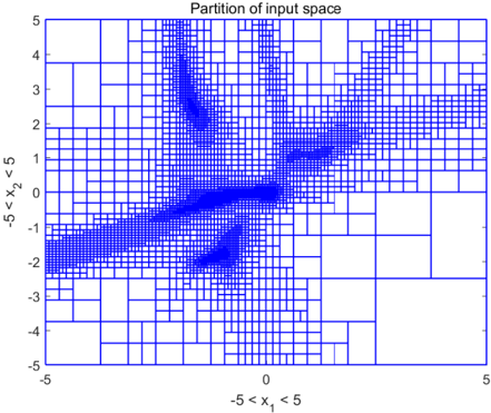
## 2D Spatial Partition Plot: Partition of input space ### Overview This image is a 2D plot illustrating a non-uniform, recursive spatial subdivision of a Cartesian coordinate system. The plot consists of a bounding box filled with blue rectangular outlines of varying sizes. The density of these rectangles varies drastically across the plot, indicating an adaptive partitioning algorithm (such as a k-d tree, quadtree, or adaptive mesh refinement) that subdivides the space more finely in specific regions of interest or high complexity, while leaving areas of low complexity as larger, undivided blocks. ### Components/Axes **Header Region:** * **Title:** "Partition of input space" (Located at the top-center of the image). **Main Chart Area:** * The core visual consists entirely of blue rectangular boxes of varying dimensions. There is no legend, as the data is represented purely by the geometric structure and density of the grid lines. **X-Axis (Bottom):** * **Label:** "-5 < x_1 < 5" (Centered below the axis). * **Scale/Markers:** Linear scale. Visible tick marks and labels are placed at: * `-5` (Bottom-left corner) * `0` (Bottom-center) * `5` (Bottom-right corner) **Y-Axis (Left):** * **Label:** "-5 < x_2 < 5" (Rotated 90 degrees counter-clockwise, centered along the left edge). * **Scale/Markers:** Linear scale. Visible tick marks and labels are placed at integer intervals: * `5` (Top-left corner) * `4`, `3`, `2`, `1` * `0` (Center-left) * `-1`, `-2`, `-3`, `-4` * `-5` (Bottom-left corner) ### Detailed Analysis *Trend Verification Note: Because this is a spatial partition plot rather than a standard line/scatter graph, "trends" are defined by the density gradients of the rectangles (transitioning from large, sparse blocks to small, dense blocks).* The input space is bounded by $x_1 \in [-5, 5]$ and $x_2 \in [-5, 5]$. The partitioning creates distinct regions of high density (very small rectangles) and low density (large rectangles). **Low-Density Regions (Sparse / Large Blocks):** These areas indicate regions where the underlying function or data requires minimal resolution. * **Bottom-Right:** The largest contiguous blocks are found in the bottom-right quadrant, roughly bounded by $x_1 > 1$ and $x_2 < -1$. * **Top-Left:** Another sparse region exists in the upper-left, roughly $x_1 < -3$ and $x_2 > 2$. * **Top-Right:** A sparse region occupies the extreme top-right corner, roughly $x_1 > 3$ and $x_2 > 3$. **High-Density Regions (Dense / Small Blocks):** These areas indicate regions of high complexity, steep gradients, or dense data clusters. The dense regions form distinct, interconnected shapes: 1. **Central-Left Band:** A dense band begins at the left edge ($x_1 = -5, x_2 \approx -1.5$) and slopes slightly upward toward the center of the plot ($x_1 \approx 0, x_2 \approx 0$). 2. **Top-Left Plume:** Branching off from the central area, a dense vertical plume extends upwards. It is centered around $x_1 \approx -1.5$ and stretches from $x_2 \approx 1$ up to the top boundary at $x_2 = 5$. 3. **Rightward Band:** From the central hub ($x_1 \approx 0, x_2 \approx 0$), another dense band extends to the right and slightly upwards, passing through $x_1 \approx 2, x_2 \approx 1$ and continuing toward the right edge at $x_1 = 5, x_2 \approx 2$. 4. **Bottom-Center Cluster:** There is a distinct, somewhat isolated dense patch located below the central hub, centered approximately at $x_1 \approx -1, x_2 \approx -2$. ### Key Observations * The partitioning is highly adaptive; the algorithm clearly targets specific topological features within the space. * The subdivisions appear to be orthogonal (axis-aligned splits), characteristic of decision trees or k-d trees. * The dense regions form a roughly star-like or branching manifold with three main arms extending from a central nexus, plus one isolated cluster. * The transition from sparse to dense is gradual in some areas (e.g., moving from the bottom-right towards the center) and abrupt in others. ### Interpretation **What the data suggests:** This image visualizes the "under the hood" mechanics of a mathematical or machine learning model. The grid represents how an algorithm has chosen to divide a 2D space to approximate a function, classify data, or solve an equation. The algorithm uses a recursive splitting method: if a region of space is "simple" (e.g., uniform data class, flat gradient), it leaves it as a large box. If a region is "complex" (e.g., a decision boundary between two classes, a steep curve in a function), it splits the box into smaller pieces to capture the fine details. **Relationship of elements:** The relationship between the large and small boxes is one of computational efficiency. By allocating tiny boxes only where necessary (the dark blue bands), the system saves memory and processing power in the empty/simple spaces (the large white boxes). **Peircean investigative / Reading between the lines:** The specific shape of the dense regions acts as a "negative space" footprint of an unseen dataset or mathematical function. * If this is a **Machine Learning Classification** model (like a Decision Tree or Random Forest), the dense blue bands represent the *decision boundaries* separating different classes of data. The algorithm is working very hard to draw precise lines between distinct clusters of data points. * If this is **Numerical Analysis** (like Adaptive Mesh Refinement for fluid dynamics or heat transfer), the dense bands represent areas of rapid change—such as a shockwave, a thermal front, or a physical boundary within the simulated space. * The isolated cluster at ($x_1 \approx -1, x_2 \approx -2$) is particularly interesting; it suggests a localized anomaly, a separate cluster of data, or a local minimum/maximum in a function that is disconnected from the main branching structure.