## Partition Plot: Partition of Input Space
### Overview
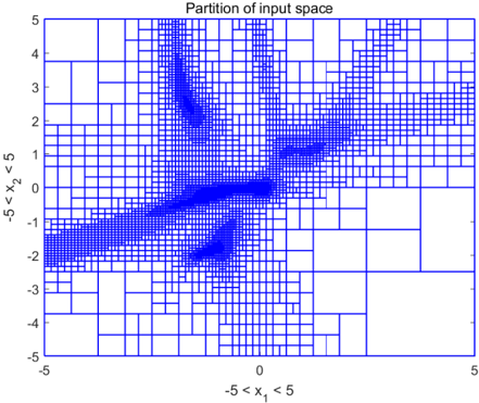
The image displays a two-dimensional partition plot titled "Partition of input space." It visualizes how a continuous 2D input space, defined by variables `x1` and `x2`, has been subdivided into a grid of rectangular regions (partitions) of varying sizes. The partitioning is non-uniform, with significantly higher density (smaller rectangles) in specific areas, suggesting an adaptive or data-driven subdivision process, common in algorithms like decision trees, adaptive mesh refinement, or certain clustering techniques.
### Components/Axes
* **Title:** "Partition of input space" (centered at the top).
* **X-Axis:**
* **Label:** `-5 < x1 < 5` (centered below the axis).
* **Scale:** Linear, ranging from -5 to 5. Major tick marks are visible at -5, 0, and 5.
* **Y-Axis:**
* **Label:** `-5 < x2 < 5` (centered to the left of the axis, rotated 90 degrees).
* **Scale:** Linear, ranging from -5 to 5. Major tick marks are visible at -5, -4, -3, -2, -1, 0, 1, 2, 3, 4, 5.
* **Visual Elements:** The entire plot area is filled with a network of blue rectangular outlines on a white background. The size of these rectangles varies dramatically across the space.
### Detailed Analysis
The partition density is highly heterogeneous. The space is divided into a mosaic of blue rectangles. The size of a rectangle is inversely proportional to the partition density in that local region.
* **High-Density Regions (Fine Partitioning):**
1. **Central Diagonal Band:** A prominent, dense band of very small rectangles runs diagonally from the lower-left quadrant (approximately `x1 ≈ -4, x2 ≈ -2`) through the origin `(0,0)` and extends into the upper-right quadrant (approximately `x1 ≈ 4, x2 ≈ 2`). This suggests a strong linear or near-linear relationship or high data density along this `x2 ≈ 0.5*x1` trend.
2. **Central Cluster:** An extremely dense cluster of the smallest rectangles is centered near the origin `(0,0)`, indicating this is the most finely resolved region of the input space.
3. **Upper-Left Cluster:** A distinct, dense cluster of small rectangles is located in the upper-left quadrant, centered approximately at `(x1 ≈ -2, x2 ≈ 3)`.
4. **Lower-Center Cluster:** Another dense cluster is located in the lower-center area, centered approximately at `(x1 ≈ -1, x2 ≈ -2)`.
* **Low-Density Regions (Coarse Partitioning):**
* The periphery of the plot, particularly the top-right corner (`x1 > 3, x2 > 3`), the bottom-right corner (`x1 > 3, x2 < -3`), and the far left edge (`x1 < -4`), is partitioned into very large rectangles. This indicates these areas are considered less important or contain little to no relevant data for the underlying model or analysis.
### Key Observations
1. **Adaptive Resolution:** The partitioning is clearly adaptive, not a uniform grid. The algorithm has allocated computational resources (smaller partitions) to specific regions of interest.
2. **Anisotropic Patterns:** The dense regions form distinct shapes—a diagonal band and several localized clusters—rather than being randomly distributed. This implies the underlying function or data distribution has specific structural features.
3. **Origin Focus:** The highest density is at the center of the coordinate system `(0,0)`, which is often a point of interest in normalized or centered data.
4. **Clear Boundaries:** The transitions between high-density and low-density regions are often abrupt, marked by a sudden increase in rectangle size.
### Interpretation
This partition plot is a visual representation of how an algorithm has "learned" or been configured to discretize a 2D input space. The patterns reveal the algorithm's focus:
* **The diagonal dense band** strongly suggests the model has identified a critical relationship or a high-density data corridor where `x2` is approximately proportional to `x1`. Predictions or calculations in this region will be more precise due to the finer grid.
* **The dense clusters** (central, upper-left, lower-center) likely correspond to areas with high concentrations of training data, complex decision boundaries, or regions where the target function exhibits high curvature or volatility. The model requires finer granularity here to capture the complexity.
* **The sparse periphery** indicates regions deemed less significant—perhaps where data is absent, the function is smooth and predictable, or the outcomes are less consequential.
In essence, this image maps the "attention" or "resolution budget" of a computational model across its input domain. It shows that the model's behavior is not uniform; it is highly tuned to specific structures and regions within the `[-5, 5] x [-5, 5]` space, with a primary focus on a central diagonal trend and several key clusters.