## [Multi-Panel Chart]: Scaling Laws for Neural Language Models
### Overview
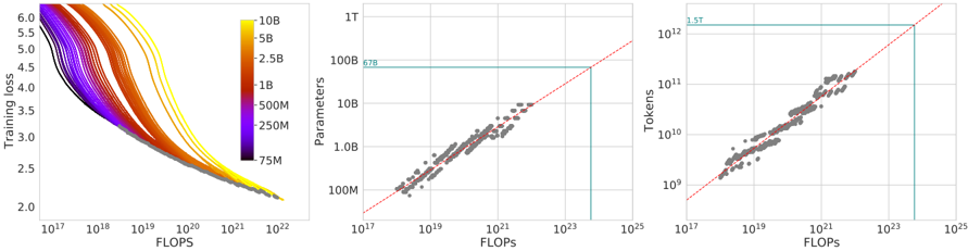
The image contains three horizontally arranged plots that collectively illustrate scaling laws in machine learning, specifically relating model size, training data, computational resources (FLOPs), and model performance (training loss). The plots use logarithmic scales on most axes to display relationships spanning several orders of magnitude.
### Components/Axes
The image is segmented into three distinct panels:
**Left Panel: Training Loss vs. FLOPs**
* **Type:** Line chart with multiple series.
* **Y-axis:** Label: "Training loss". Scale: Linear, from 2.0 to 6.0.
* **X-axis:** Label: "FLOPs". Scale: Logarithmic, from 10¹⁷ to 10²².
* **Legend:** Positioned on the right side of the plot. It maps line colors to model parameter counts. From top (yellow) to bottom (dark purple): 10B, 5B, 2.5B, 1B, 500M, 250M, 75M.
* **Data Series:** Multiple colored lines, each representing a model of a specific size (as per legend), plotting training loss as a function of total floating-point operations (FLOPs).
**Middle Panel: Parameters vs. FLOPs**
* **Type:** Scatter plot with trend line.
* **Y-axis:** Label: "Parameters". Scale: Logarithmic, from 100M to 1T (1 Trillion).
* **X-axis:** Label: "FLOPs". Scale: Logarithmic, from 10¹⁷ to 10²⁵.
* **Key Annotations:**
* A red dashed line representing a power-law trend.
* A horizontal teal line intersecting the y-axis at approximately **67B** (labeled "67B" in teal text).
* A vertical teal line intersecting the x-axis at approximately **10²⁴** FLOPs.
* **Data Points:** Grey diamond-shaped markers representing individual model training runs.
**Right Panel: Tokens vs. FLOPs**
* **Type:** Scatter plot with trend line.
* **Y-axis:** Label: "Tokens". Scale: Logarithmic, from 10⁹ to 10¹².
* **X-axis:** Label: "FLOPs". Scale: Logarithmic, from 10¹⁷ to 10²⁵.
* **Key Annotations:**
* A red dashed line representing a power-law trend.
* A horizontal teal line intersecting the y-axis at approximately **5.5T** (labeled "5.5T" in teal text).
* A vertical teal line intersecting the x-axis at approximately **10²⁴** FLOPs.
* **Data Points:** Grey diamond-shaped markers representing individual model training runs.
### Detailed Analysis
**Left Panel (Training Loss vs. FLOPs):**
* **Trend Verification:** All lines slope downward from left to right, indicating that training loss decreases as the number of FLOPs (compute) increases.
* **Data Series Analysis:** For a fixed amount of compute (a vertical line), larger models (e.g., 10B, yellow line) consistently achieve lower training loss than smaller models (e.g., 75M, dark purple line). The curves for larger models are positioned lower and to the left, showing they are more compute-efficient at reaching a given loss level.
* **Approximate Values:** At 10²⁰ FLOPs, the 10B model has a loss of ~2.5, while the 75M model has a loss of ~4.0. All curves show diminishing returns, flattening as FLOPs increase.
**Middle Panel (Parameters vs. FLOPs):**
* **Trend Verification:** The data points cluster tightly around the red dashed trend line, which slopes upward. This indicates a strong positive correlation: models trained with more FLOPs tend to have more parameters.
* **Key Data Point:** The teal lines highlight a specific configuration: a model with **~67 billion parameters** trained using approximately **10²⁴ FLOPs**.
* **Relationship:** The log-log plot suggests a power-law relationship between model size and required compute.
**Right Panel (Tokens vs. FLOPs):**
* **Trend Verification:** The data points cluster tightly around the red dashed trend line, which slopes upward. This indicates a strong positive correlation: training runs using more FLOPs process more tokens (data).
* **Key Data Point:** The teal lines highlight a specific configuration: a training run consuming **~5.5 trillion tokens** used approximately **10²⁴ FLOPs**.
* **Relationship:** The log-log plot suggests a power-law relationship between the amount of training data and required compute.
### Key Observations
1. **Consistent Scaling:** All three plots demonstrate clear, predictable scaling relationships. Performance (lower loss) improves with more compute, which in turn is used to train larger models on more data.
2. **Compute Allocation:** The middle and right plots together imply a relationship between model size (Parameters) and data size (Tokens) for a given compute budget (FLOPs). The highlighted point (67B Params, 5.5T Tokens, 10²⁴ FLOPs) represents one such allocation.
3. **Efficiency:** The left plot shows that simply adding more compute to a small model yields diminishing returns. To achieve significantly lower loss, one must increase the model size (move to a different colored curve).
4. **Data Density:** The scatter plots (middle and right) show a high density of data points in the range of 10¹⁹ to 10²² FLOPs, suggesting this is a common region for experimental model training.
### Interpretation
This set of charts provides a visual foundation for the "scaling laws" observed in large language model training. The data suggests that model performance (training loss) is a predictable function of three key factors: **model size (parameters)**, **dataset size (tokens)**, and **compute budget (FLOPs)**.
The relationships are not linear but follow power laws, meaning that to achieve a linear improvement in loss, one needs an exponential increase in resources. The teal annotations likely point to a specific model configuration of interest (e.g., a 67B parameter model trained on 5.5T tokens), showing the compute required to train it.
The overarching message is that progress in model capability is driven by scaling these three factors in a balanced way. The charts serve as a guide for researchers to estimate the resources required to reach a target performance level or to understand the trade-offs between building a larger model versus training a smaller model on more data. The tight clustering of points around the trend lines indicates these scaling laws are robust and reliable for planning large-scale training runs.