## Diagram: Algorithm for Generating Grid Patterns from Input Images
### Overview
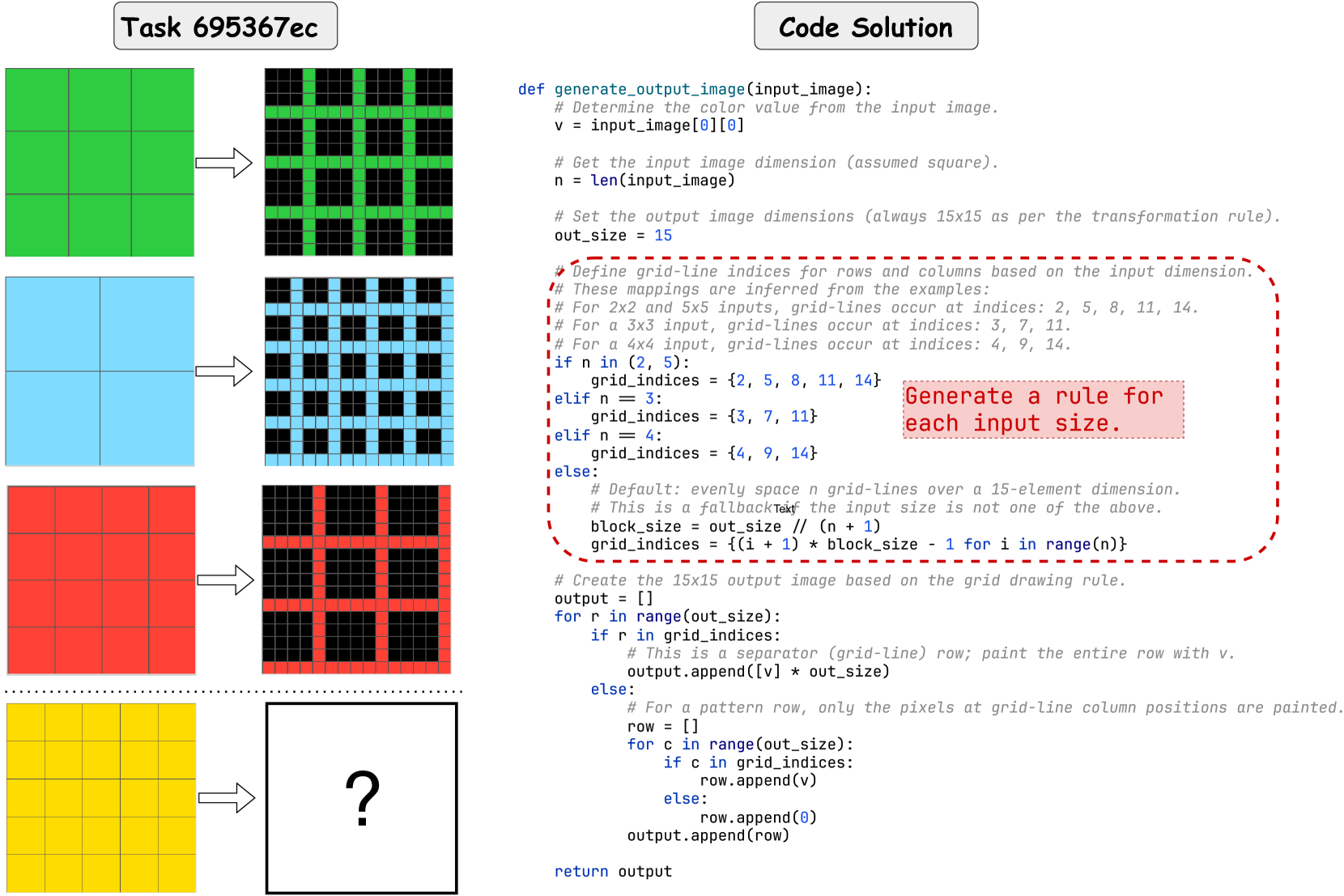
The image presents a technical diagram illustrating a programming task (labeled "Task 695367ec") and its corresponding "Code Solution." It visually demonstrates a transformation rule where simple, solid-colored input grids are converted into complex, patterned output grids. The right side contains the Python code that implements this transformation. The final example (a yellow 5x5 grid) has a question mark, indicating the output is to be determined by applying the provided algorithm.
### Components/Axes
The image is divided into two primary sections:
1. **Left Section (Visual Examples):**
* **Structure:** Four rows, each showing an input grid (left), an arrow, and the resulting output grid (right).
* **Input Grids:** Solid-colored squares with visible grid lines indicating their dimensions.
* Row 1: Green 3x3 grid.
* Row 2: Blue 2x2 grid.
* Row 3: Red 4x4 grid.
* Row 4: Yellow 5x5 grid (output is a white box with a black question mark).
* **Output Grids:** 15x15 pixel grids with a black background. Colored pixels (matching the input color) form a pattern of intersecting horizontal and vertical lines, creating a "grid of grids" effect. The pattern density varies with the input size.
2. **Right Section (Code Solution):**
* **Title:** "Code Solution" in a rounded rectangle.
* **Content:** A Python function definition `def generate_output_image(input_image):` with extensive comments.
* **Highlighted Region:** A red dashed box surrounds the core logic for determining grid-line positions, with an attached note: "Generate a rule for each input size."
### Detailed Analysis
**Code Transcription and Logic:**
The Python function `generate_output_image` takes a 2D list (`input_image`) representing the input grid. The algorithm proceeds as follows:
1. **Extract Color:** `v = input_image[0][0]` – The color value (e.g., green, blue) is taken from the top-left pixel of the input.
2. **Determine Input Size:** `n = len(input_image)` – Assumes the input is square.
3. **Set Output Size:** `out_size = 15` – The output is always a 15x15 grid.
4. **Define Grid Indices (Core Rule):** This is the critical step, highlighted in the diagram. The code sets a list `grid_indices` that defines which rows and columns in the 15x15 output will be painted with the color `v`.
* For `n` (input size) of 2 or 5: `grid_indices = {2, 5, 8, 11, 14}`
* For `n = 3`: `grid_indices = {3, 7, 11}`
* For `n = 4`: `grid_indices = {4, 9, 14}`
* **Fallback Rule (for other `n`):** `block_size = out_size // (n + 1)`, then `grid_indices = {(i + 1) * block_size - 1 for i in range(n)}`. This evenly spaces `n` grid lines within the 15-element dimension.
5. **Generate Output:** The code iterates through each row `r` of the 15x15 output.
* If `r` is in `grid_indices`, the entire row is filled with color `v` (creating a horizontal separator line).
* Otherwise, it creates a row where only the pixels at column indices `c` that are in `grid_indices` are painted with `v` (creating the vertical segments of the pattern).
**Visual Pattern Verification:**
* **3x3 Input (Green):** Output shows green lines at rows/columns 3, 7, and 11, creating a 2x2 arrangement of large black squares within the 15x15 grid.
* **2x2 Input (Blue):** Output shows blue lines at rows/columns 2, 5, 8, 11, and 14, creating a denser 5x5 arrangement of small black squares.
* **4x4 Input (Red):** Output shows red lines at rows/columns 4, 9, and 14, creating a 3x3 arrangement of black squares.
* **5x5 Input (Yellow):** According to the code rule for `n=5`, the output should have yellow lines at indices {2, 5, 8, 11, 14}, identical to the pattern for the 2x2 input but in yellow.
### Key Observations
1. **Fixed Output Dimension:** Regardless of input size (2x2 to 5x5), the output is always rendered in a 15x15 pixel space.
2. **Discrete Rule Set:** The algorithm uses a lookup table for common input sizes (2,3,4,5) rather than a single mathematical formula, suggesting these were the specific cases defined for the task.
3. **Pattern Inversion:** The output is essentially a "wireframe" or "grid overlay" of the input's structure, but scaled and positioned within a fixed canvas. The black squares in the output represent the "cells" of the original input grid.
4. **Size-to-Pattern Mapping:** The relationship is not linear. Both 2x2 and 5x5 inputs produce the same spatial frequency of grid lines (indices {2,5,8,11,14}), while 3x3 and 4x4 produce different, coarser patterns.
### Interpretation
This diagram explains a **visual programming puzzle or algorithm challenge**. The core task is to infer a transformation rule from examples and implement it. The "rule" is the mapping from an input grid's dimension (`n`) to a specific set of coordinates (`grid_indices`) in a fixed-size output canvas.
The provided solution reveals that the rule is **empirical and case-based** for the given examples, with a general fallback. The interesting anomaly is that the 2x2 and 5x5 inputs share the same output pattern geometry. This suggests the rule might be designed to create a visually distinct pattern for each input size within the constraints of a 15x15 output, but the mapping for 2 and 5 converges. The question mark for the 5x5 yellow grid tests the viewer's ability to apply the stated rule: since `n=5` is explicitly handled, its output should be a yellow version of the blue 2x2 pattern.
The diagram serves as both a problem statement (left) and its solution (right), emphasizing the importance of precise rule extraction and implementation in computational thinking. The highlighted code section underscores that the heart of the problem is defining the `grid_indices` for each input size.