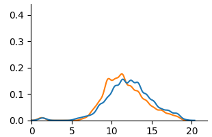
## Density Plot: Distribution Comparison ### Overview The image is a density plot comparing two distributions, one represented by a blue line and the other by an orange line. The plot shows the probability density of each distribution across a range of values from approximately 0 to 20. ### Components/Axes * **X-axis:** Ranges from 0 to 20, with tick marks at 0, 5, 10, 15, and 20. * **Y-axis:** Ranges from 0.0 to 0.4, with tick marks at 0.0, 0.1, 0.2, 0.3, and 0.4. * **Blue Line:** Represents one distribution. * **Orange Line:** Represents another distribution. ### Detailed Analysis * **Blue Line:** * Starts near 0.0 at x=0. * Gradually increases to a peak around x=11, reaching a density of approximately 0.16. * Decreases to near 0.0 around x=20. * **Orange Line:** * Starts near 0.0 at x=0. * Gradually increases to a peak around x=12, reaching a density of approximately 0.18. * Decreases to near 0.0 around x=20. ### Key Observations * Both distributions are unimodal (have one peak). * The orange distribution has a slightly higher peak density than the blue distribution. * The peaks of the two distributions are close to each other, with the orange distribution's peak slightly to the right of the blue distribution's peak. * Both distributions have similar shapes, with a slight right skew. ### Interpretation The density plot compares two distributions, showing their relative probabilities across a range of values. The orange distribution has a slightly higher probability density around x=12 compared to the blue distribution around x=11. Both distributions have similar shapes and ranges, suggesting they represent similar phenomena with slightly different central tendencies. The plot indicates that values around 11 and 12 are more likely to occur in these distributions compared to values at the extremes (near 0 or 20).