## Scatter Plots: Interaural Phase Difference (IPD) and Interaural Level Difference (ILD) vs. Peak Frequency
### Overview
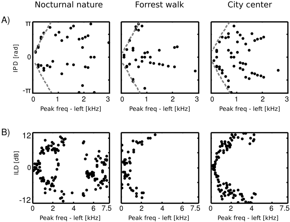
The image presents six scatter plots arranged in a 2x3 grid. The plots visualize the relationship between peak frequency (on the x-axis) and either Interaural Phase Difference (IPD) or Interaural Level Difference (ILD) (on the y-axis) for three different acoustic environments: Nocturnal nature, Forrest walk, and City center. Each environment is represented by two plots – one for IPD and one for ILD. A dashed grey line is overlaid on each of the top row plots.
### Components/Axes
* **X-axis (all plots):** Peak freq - left [kHz]. Scale ranges from 0 to 3 kHz for the top row plots (IPD) and 0 to 7.5 kHz for the bottom row plots (ILD).
* **Y-axis (top row plots):** IPD [rad]. Scale ranges from approximately -π to π.
* **Y-axis (bottom row plots):** ILD [dB]. Scale ranges from approximately -1.2 to 12 dB.
* **Titles (top row):** Nocturnal nature, Forrest walk, City center.
* **Labels (left side):** A) and B) to distinguish the IPD and ILD plots.
* **Data Points:** Black dots representing individual data points.
* **Overlaid Line:** Dashed grey line present in all three IPD plots.
### Detailed Analysis or Content Details
**A) IPD vs. Peak Frequency**
* **Nocturnal Nature:** The data points generally cluster between 0.2 and 2.5 kHz. The trend shows a positive correlation between peak frequency and IPD up to approximately 1.5 kHz, after which the IPD values become more scattered and decrease. Approximate data points: (0.3 kHz, 0.3 rad), (1.0 kHz, 1.5 rad), (2.0 kHz, 0.1 rad).
* **Forrest Walk:** Similar to Nocturnal Nature, the data points are concentrated between 0.2 and 2.5 kHz. The trend also shows a positive correlation between peak frequency and IPD up to approximately 1.5 kHz, followed by more scattered data. Approximate data points: (0.4 kHz, 0.4 rad), (1.2 kHz, 1.7 rad), (2.2 kHz, 0.2 rad).
* **City Center:** Data points are distributed between 0.2 and 3.0 kHz. The positive correlation between peak frequency and IPD is observed up to approximately 1.5 kHz, but the scatter is more pronounced than in the other two environments. Approximate data points: (0.5 kHz, 0.5 rad), (1.4 kHz, 1.8 rad), (2.8 kHz, -0.1 rad). The dashed grey line appears to approximate the trend of the data.
**B) ILD vs. Peak Frequency**
* **Nocturnal Nature:** Data points are spread between 0.5 and 6.5 kHz. There's a slight positive correlation between peak frequency and ILD up to approximately 2 kHz, after which the ILD values become more variable. Approximate data points: (1.0 kHz, 1.0 dB), (3.0 kHz, 2.0 dB), (5.0 kHz, 0.5 dB).
* **Forrest Walk:** Data points are distributed between 0.5 and 7.0 kHz. A similar trend to Nocturnal Nature is observed, with a slight positive correlation up to approximately 2 kHz. Approximate data points: (0.8 kHz, 0.8 dB), (2.5 kHz, 2.5 dB), (6.0 kHz, 0.2 dB).
* **City Center:** Data points are spread between 0.5 and 7.5 kHz. A positive correlation between peak frequency and ILD is visible up to approximately 3 kHz, followed by a decrease in ILD. Approximate data points: (1.2 kHz, 2.0 dB), (3.5 kHz, 4.0 dB), (6.5 kHz, -0.5 dB).
### Key Observations
* The IPD plots all exhibit a similar trend of increasing IPD with increasing peak frequency up to a certain point, followed by a decrease or increased scatter.
* The ILD plots show a more subtle positive correlation between peak frequency and ILD, with more variability in the data.
* The City Center environment appears to have the most scattered data points in both IPD and ILD plots, suggesting a more complex acoustic environment.
* The dashed grey line in the IPD plots seems to represent a general trend of the data, but doesn't perfectly fit all data points.
### Interpretation
The data suggests that the acoustic environments influence the relationship between peak frequency and interaural cues (IPD and ILD). The consistent trend in the IPD plots indicates that lower frequencies are generally associated with larger interaural phase differences, which is consistent with the physics of sound wave propagation. The differences between the environments suggest that the complexity of the soundscape affects the precision of these cues. The City Center, with its more scattered data, likely has more reflections and reverberations, making it harder to determine the precise location of sound sources. The ILD plots, while showing a less pronounced trend, suggest that higher frequencies are associated with larger interaural level differences, which is also expected due to the head-shadow effect. The overlaid dashed line in the IPD plots could represent a model or expectation of the IPD-frequency relationship, against which the observed data is compared. The differences between the observed data and the model could reveal insights into the specific acoustic characteristics of each environment.