\n
## Diagram: Diffusion Sliding Window and Trajectory Analysis
### Overview
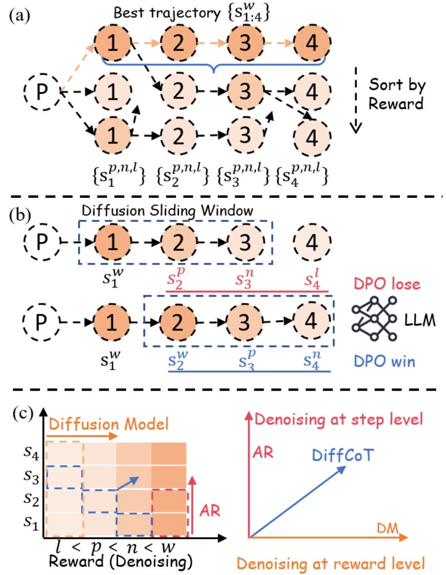
The image presents a diagram illustrating a diffusion sliding window approach for reinforcement learning, likely within the context of Direct Preference Optimization (DPO). It compares a "Best Trajectory" approach with a "Diffusion Sliding Window" method, and then visualizes the underlying diffusion model. The diagram is divided into three sections: (a) Best Trajectory, (b) Diffusion Sliding Window, and (c) Diffusion Model.
### Components/Axes
* **Section (a): Best Trajectory**
* Nodes labeled 1, 2, 3, and 4 representing states.
* Circles representing the "Best Trajectory" {s<sub>1:4</sub>}.
* Parentheses representing initial state P.
* Braces containing state sequences {s<sub>1</sub><sup>p,n,l</sup>}, {s<sub>2</sub><sup>p,n,l</sup>}, {s<sub>3</sub><sup>p,n,l</sup>}, {s<sub>4</sub><sup>p,n,l</sup>}.
* An arrow labeled "Sort by Reward" pointing downwards.
* **Section (b): Diffusion Sliding Window**
* Nodes labeled 1, 2, 3, and 4 representing states.
* Circles representing state sequences s<sub>1</sub><sup>w</sup>, s<sub>2</sub><sup>w</sup>, s<sub>3</sub><sup>w</sup>, s<sub>4</sub><sup>w</sup>.
* Parentheses representing initial state P.
* States labeled with superscripts 'p' and 'n' (s<sub>1</sub><sup>p</sup>, s<sub>2</sub><sup>p</sup>, s<sub>3</sub><sup>n</sup>, s<sub>4</sub><sup>n</sup>).
* States labeled with 'l' (s<sub>4</sub><sup>l</sup>).
* A legend indicating "DPO lose" (red) and "DPO win" (blue) represented by a tangled line graph labeled "LLM".
* **Section (c): Diffusion Model**
* Vertical axis labeled "Reward (Denoising)".
* Horizontal axis labeled "Denoising at reward level".
* States labeled S<sub>1</sub>, S<sub>2</sub>, S<sub>3</sub>, and S<sub>4</sub>.
* A heatmap representing the diffusion model.
* Lines representing "AR" (AutoRegressive) and "DiffCoT" (Diffusion Chain of Thought).
* "DM" label.
### Detailed Analysis or Content Details
**Section (a): Best Trajectory**
The diagram shows a sequence of states 1, 2, 3, and 4 forming the best trajectory. The initial state is denoted by P. Below this, multiple possible trajectories are shown, each starting from P and leading to the states 1 through 4, labeled with {s<sub>1</sub><sup>p,n,l</sup>}, {s<sub>2</sub><sup>p,n,l</sup>}, {s<sub>3</sub><sup>p,n,l</sup>}, {s<sub>4</sub><sup>p,n,l</sup>}. The arrow "Sort by Reward" indicates that these trajectories are ranked based on their associated rewards.
**Section (b): Diffusion Sliding Window**
This section illustrates the diffusion sliding window approach. Two trajectories are shown, starting from P. The first trajectory is labeled s<sub>1</sub><sup>w</sup>, s<sub>2</sub><sup>w</sup>, s<sub>3</sub><sup>w</sup>, s<sub>4</sub><sup>w</sup>. The second trajectory has states labeled with 'p' and 'n' indicating preference. s<sub>1</sub><sup>p</sup>, s<sub>2</sub><sup>p</sup>, s<sub>3</sub><sup>n</sup>, s<sub>4</sub><sup>n</sup>. The state s<sub>4</sub><sup>l</sup> is also shown. The legend indicates that the red lines represent "DPO lose" and the blue lines represent "DPO win", visualized as a complex line graph labeled "LLM".
**Section (c): Diffusion Model**
The heatmap shows the diffusion model's representation of reward. The vertical axis represents the reward level, and the horizontal axis represents the denoising level. The states S<sub>1</sub>, S<sub>2</sub>, S<sub>3</sub>, and S<sub>4</sub> are positioned along the vertical axis. The heatmap is shaded, with darker shades indicating higher values. The line labeled "AR" slopes upwards, and the line labeled "DiffCoT" also slopes upwards, but with a steeper gradient. The point where the lines intersect is labeled "DM". The x-axis is labeled "Denoising at step level" and the y-axis is labeled "Reward (Denoising)". The inequality l < p < n < w is shown along the y-axis.
### Key Observations
* The "Best Trajectory" section highlights the concept of selecting the optimal path based on reward.
* The "Diffusion Sliding Window" section introduces a method for exploring multiple trajectories and evaluating their preferences (DPO win/lose).
* The "Diffusion Model" section visualizes how the model represents reward and denoising levels.
* The heatmap in section (c) suggests a correlation between reward and denoising.
* The lines AR and DiffCoT represent different approaches to denoising, with DiffCoT exhibiting a stronger relationship between denoising and reward.
### Interpretation
The diagram illustrates a novel approach to reinforcement learning using diffusion models and Direct Preference Optimization (DPO). The "Diffusion Sliding Window" method appears to be a way to sample multiple trajectories and learn from preferences, as indicated by the "DPO win/lose" labels. The diffusion model, visualized in section (c), provides a representation of the reward landscape, allowing for more informed denoising and trajectory selection. The comparison between "AR" and "DiffCoT" suggests that the latter approach is more effective at capturing the relationship between denoising and reward. The inequality l < p < n < w likely represents a ranking or ordering of different parameters or stages within the diffusion process. The overall goal seems to be to improve the efficiency and effectiveness of reinforcement learning by leveraging the power of diffusion models and preference-based learning. The diagram suggests a system where the LLM is used to determine the preference between trajectories, and this information is then used to refine the diffusion model. The heatmap in section (c) is a visual representation of the model's understanding of the reward function.