## Line Graph: Plot of (1 - std(X)) / std(X) for Bernoulli(p)
### Overview
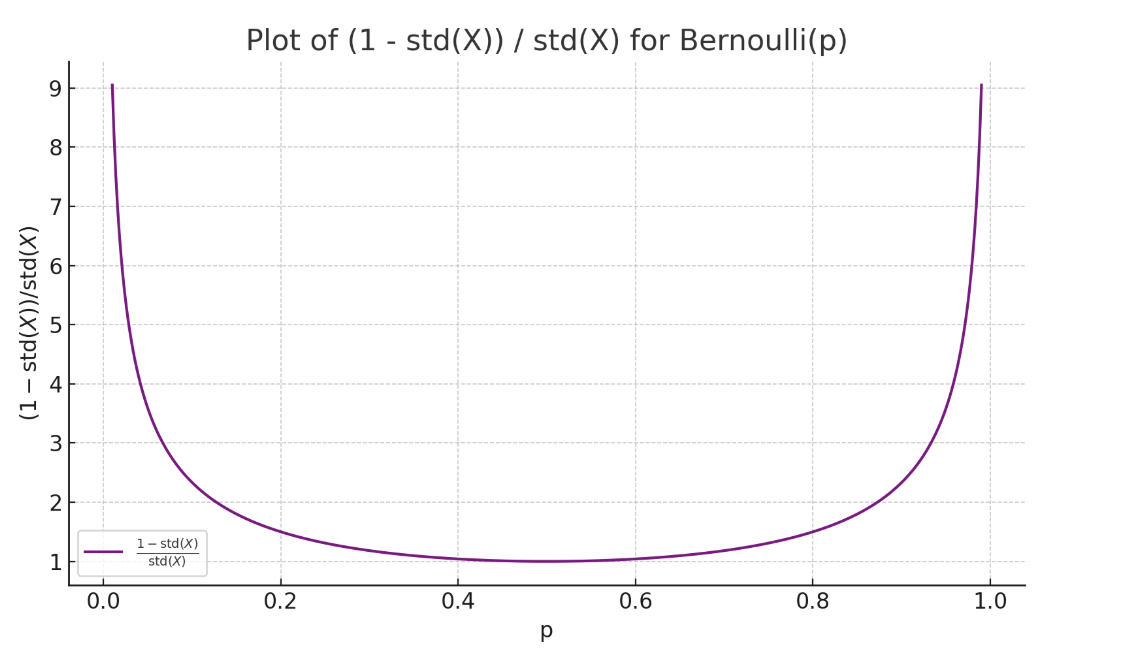
The image is a single-line graph plotting a mathematical function related to the Bernoulli distribution. The graph shows a symmetric, U-shaped curve that reaches its minimum value at the center of the x-axis range and increases asymptotically towards both ends.
### Components/Axes
* **Title:** "Plot of (1 - std(X)) / std(X) for Bernoulli(p)"
* **X-Axis:**
* **Label:** "p"
* **Scale:** Linear, ranging from 0.0 to 1.0.
* **Major Tick Marks:** 0.0, 0.2, 0.4, 0.6, 0.8, 1.0.
* **Y-Axis:**
* **Label:** "(1 - std(X))/std(X)"
* **Scale:** Linear, ranging from 1 to 9.
* **Major Tick Marks:** 1, 2, 3, 4, 5, 6, 7, 8, 9.
* **Legend:**
* **Position:** Bottom-left corner of the plot area.
* **Content:** A purple line segment followed by the text "1 - std(X) / std(X)".
* **Data Series:**
* A single, continuous, solid purple line.
* **Grid:** Light gray, dashed grid lines are present for both major x and y ticks.
### Detailed Analysis
The plotted function is `(1 - std(X)) / std(X)`, where `X` is a Bernoulli random variable with parameter `p`. The standard deviation of a Bernoulli(p) variable is `sqrt(p*(1-p))`.
**Trend Verification:** The curve is symmetric around `p = 0.5`. It starts at a very high value near `p = 0`, decreases to a minimum at `p = 0.5`, and then increases symmetrically to a very high value near `p = 1`.
**Approximate Data Points (Visual Estimation):**
* At `p = 0.5`: The curve reaches its minimum. The y-value is approximately **1.0**.
* At `p = 0.2` and `p = 0.8`: The y-value is approximately **1.5**.
* At `p = 0.1` and `p = 0.9`: The y-value is approximately **2.2**.
* At `p = 0.05` and `p = 0.95`: The y-value is approximately **4.0**.
* Near `p = 0.01` and `p = 0.99`: The y-value approaches or exceeds the upper limit of the graph (**9.0**).
### Key Observations
1. **Symmetry:** The graph is perfectly symmetric about the vertical line `p = 0.5`.
2. **Minimum Point:** The function achieves its global minimum value of approximately 1.0 at `p = 0.5`.
3. **Asymptotic Behavior:** The function value increases without bound (asymptotically) as `p` approaches 0 or 1. The graph is clipped at y=9, but the trend indicates it would continue to rise sharply.
4. **Monotonicity:** The function is strictly decreasing on the interval `p ∈ (0, 0.5]` and strictly increasing on the interval `p ∈ [0.5, 1)`.
### Interpretation
This graph visualizes the behavior of the ratio `(1 - σ) / σ` (where σ is the standard deviation) for a Bernoulli distribution as its success probability `p` varies.
* **Mathematical Meaning:** The expression simplifies to `1/σ - 1`. Since `σ = sqrt(p(1-p))`, the plotted function is `1/sqrt(p(1-p)) - 1`. The graph confirms that this value is minimized when `p(1-p)` is maximized, which occurs at `p=0.5`.
* **Statistical Insight:** The standard deviation of a Bernoulli variable is maximized at `p=0.5` (where `σ = 0.5`). At this point, the ratio `(1 - 0.5)/0.5 = 1`. As `p` moves towards 0 or 1, the distribution becomes more certain (σ decreases), causing the ratio `1/σ - 1` to grow very large. The graph thus illustrates how the "relative deviation" (as defined by this specific ratio) explodes as the Bernoulli process becomes nearly deterministic.
* **Visual Pattern:** The pronounced U-shape highlights the extreme sensitivity of this ratio to values of `p` near the boundaries (0 and 1), contrasting with its stable, minimal value at the point of maximum uncertainty (`p=0.5`).