## Histogram Plots: Conductance Distributions
### Overview
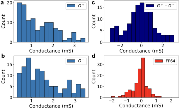
The image presents four histogram plots (a, b, c, d) displaying the distribution of conductance values in milliSiemens (mS) for different experimental conditions or data sets. Each plot shows the count (frequency) of observations for various conductance ranges.
### Components/Axes
* **General Structure:** Each plot has a similar structure:
* **Y-axis:** "Count", ranging from 0 to a maximum value (varying between plots).
* **X-axis:** "Conductance (mS)", with varying ranges depending on the plot.
* **Legend:** Located in the top-right corner of each plot, indicating the data series represented.
* **Plot a:**
* **Y-axis:** Count, ranging from 0 to 20.
* **X-axis:** Conductance (mS), ranging from 0 to 3.
* **Legend:** "G+" (dark blue).
* **Plot b:**
* **Y-axis:** Count, ranging from 0 to 15.
* **X-axis:** Conductance (mS), ranging from 0 to 3.
* **Legend:** "G-" (dark blue).
* **Plot c:**
* **Y-axis:** Count, ranging from 0 to 15.
* **X-axis:** Conductance (mS), ranging from -2 to 2.
* **Legend:** "G+ - G-" (dark blue).
* **Plot d:**
* **Y-axis:** Count, ranging from 0 to 30.
* **X-axis:** Conductance (mS), ranging from -2 to 2.
* **Legend:** "FP64" (red).
### Detailed Analysis
* **Plot a (G+):**
* The distribution is right-skewed, with the highest count occurring between 0 and 1 mS.
* Approximate counts:
* 0-0.5 mS: ~20
* 0.5-1 mS: ~19
* 1-1.5 mS: ~12
* 1.5-2 mS: ~9
* 2-2.5 mS: ~10
* 2.5-3 mS: ~3
* 3-3.5 mS: ~7
* **Plot b (G-):**
* The distribution is also right-skewed, similar to Plot a.
* Approximate counts:
* 0-0.5 mS: ~11
* 0.5-1 mS: ~17
* 1-1.5 mS: ~13
* 1.5-2 mS: ~13
* 2-2.5 mS: ~5
* 2.5-3 mS: ~4
* 3-3.5 mS: ~8
* **Plot c (G+ - G-):**
* The distribution is centered around 0 mS, with a relatively symmetrical shape.
* Approximate counts:
* -2 to -1.5 mS: ~3
* -1.5 to -1 mS: ~7
* -1 to -0.5 mS: ~8
* -0.5 to 0 mS: ~14
* 0 to 0.5 mS: ~15
* 0.5 to 1 mS: ~8
* 1 to 1.5 mS: ~7
* 1.5 to 2 mS: ~3
* **Plot d (FP64):**
* The distribution is sharply peaked around 0 mS.
* Approximate counts:
* -2 to -1.5 mS: ~1
* -1.5 to -1 mS: ~2
* -1 to -0.5 mS: ~6
* -0.5 to 0 mS: ~14
* 0 to 0.5 mS: ~28
* 0.5 to 1 mS: ~7
* 1 to 1.5 mS: ~3
* 1.5 to 2 mS: ~1
### Key Observations
* Plots a (G+) and b (G-) show similar distributions, both skewed towards lower conductance values.
* Plot c (G+ - G-) shows a distribution centered around zero, suggesting a balance between G+ and G- values.
* Plot d (FP64) exhibits a much narrower distribution, with a strong peak at 0 mS, indicating a more consistent conductance value for this condition.
### Interpretation
The histograms provide insights into the conductance characteristics of different experimental conditions. The similarity between G+ and G- distributions suggests a common underlying mechanism. The G+ - G- distribution centered around zero implies a degree of compensation or balance between these two components. The sharp peak in the FP64 distribution indicates a more stable and defined conductance state compared to the other conditions. The data suggests that FP64 exhibits a more consistent conductance behavior, while G+ and G- have a broader range of conductance values. The difference between G+ and G- is relatively centered around zero, suggesting that they tend to balance each other out.