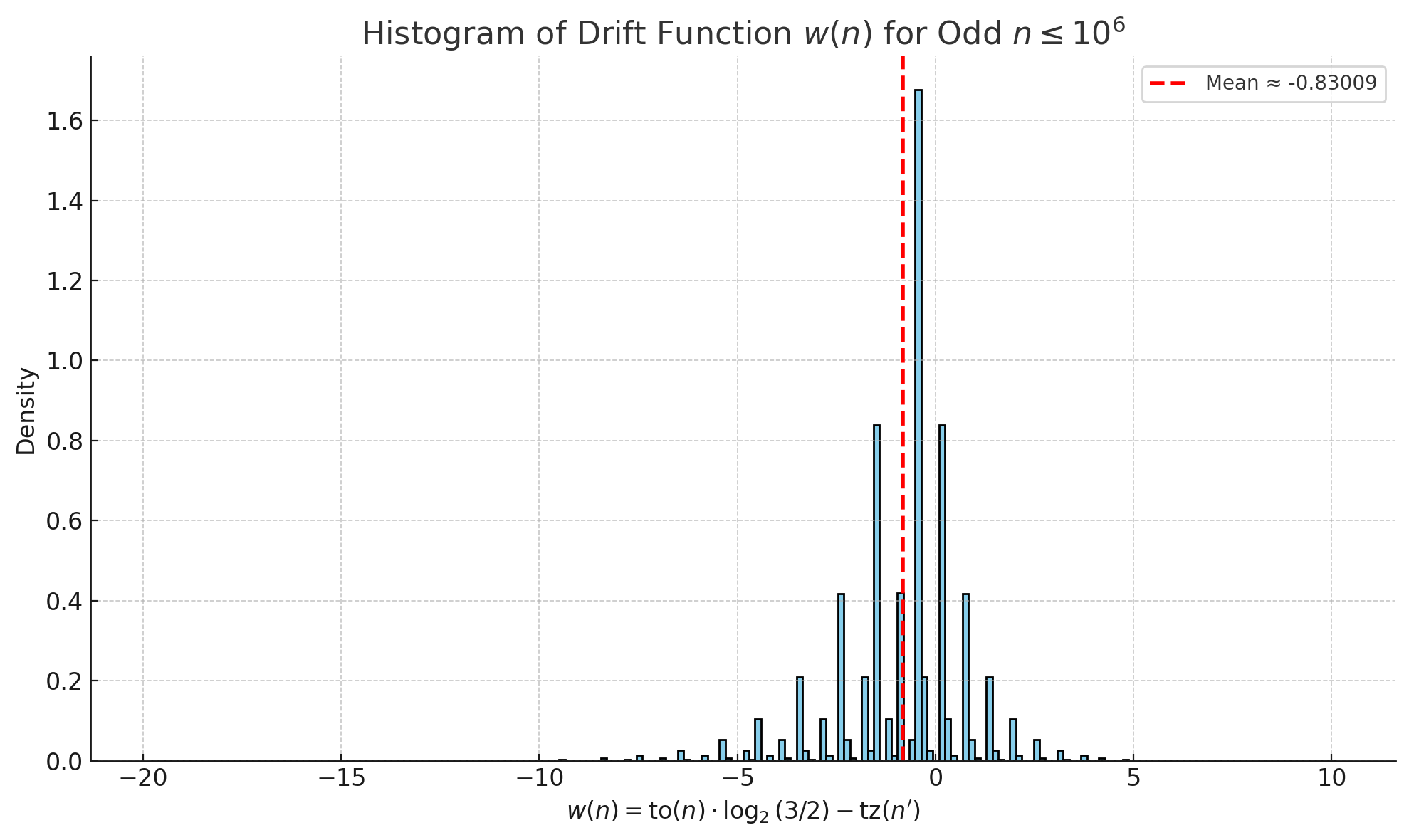
## Histogram: Drift Function w(n) for Odd n ≤ 10⁶ ### Overview The image displays a histogram visualizing the distribution of the drift function \( w(n) \) for odd integers \( n \leq 10^6 \). The histogram is centered around \( w(n) = 0 \), with a notable peak at this value. A red dashed line indicates the mean of the distribution, labeled as approximately \( -0.83009 \). The x-axis spans from \( -20 \) to \( 10 \), while the y-axis (density) ranges up to \( 1.6 \). --- ### Components/Axes - **Title**: "Histogram of Drift Function \( w(n) \) for Odd \( n \leq 10^6 \)" - **X-axis**: - Label: \( w(n) = \text{to}(n) \cdot \log_2(3/2) - \text{tz}(n') \) - Range: \( -20 \) to \( 10 \) - Tick marks: Incremented by \( 5 \) units. - **Y-axis**: - Label: "Density" - Range: \( 0 \) to \( 1.6 \) - Tick marks: Incremented by \( 0.2 \) units. - **Legend**: - Position: Top-right corner. - Content: Red dashed line labeled "Mean ≈ -0.83009". --- ### Detailed Analysis - **Histogram Bars**: - Blue bars represent the frequency distribution of \( w(n) \). - **Peak**: The tallest bar is centered at \( w(n) = 0 \), with a density of approximately \( 1.6 \). - **Symmetry**: The distribution is roughly symmetric around \( 0 \), but slightly skewed left due to the mean being negative. - **Spread**: - Left tail: Extends to \( w(n) \approx -20 \), with density dropping to near \( 0 \). - Right tail: Extends to \( w(n) \approx 10 \), with density also near \( 0 \). - **Notable Features**: - A secondary peak near \( w(n) \approx 2 \) with density ~\( 0.8 \). - A sharp drop in density between \( w(n) = -5 \) and \( w(n) = 0 \). - **Mean Line**: - Red dashed line at \( w(n) \approx -0.83009 \), slightly left of the central peak. --- ### Key Observations 1. **Central Concentration**: Most values of \( w(n) \) cluster tightly around \( 0 \), indicating a high frequency of near-zero drift. 2. **Skewness**: The mean (\( -0.83009 \)) is slightly left of the peak, suggesting a mild leftward bias in the distribution. 3. **Long Tails**: The distribution has heavy tails, with non-zero density extending to \( \pm 20 \), though these regions are sparsely populated. 4. **Secondary Peak**: A smaller peak near \( w(n) = 2 \) may indicate a secondary mode or clustering of specific \( n \)-values. --- ### Interpretation The histogram demonstrates that the drift function \( w(n) \) for odd \( n \leq 10^6 \) is predominantly centered around \( 0 \), with a slight negative bias in its mean. This suggests that, on average, the drift function exhibits a tendency toward negative values, though the majority of individual \( w(n) \) values are close to zero. The heavy tails imply that extreme drift values (both positive and negative) occur infrequently but are not impossible. The secondary peak near \( w(n) = 2 \) warrants further investigation to determine if it corresponds to a specific subset of \( n \)-values or a systematic pattern in the drift function. The red dashed mean line confirms the calculated average, aligning with the visual skew. The distribution’s shape (approximately symmetric with a slight leftward tilt) may reflect underlying properties of the functions \( \text{to}(n) \), \( \log_2(3/2) \), and \( \text{tz}(n') \), though additional context about these components is required for deeper analysis.