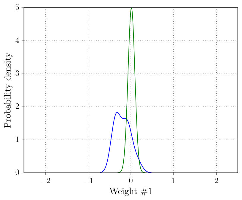
# Technical Document Extraction: Probability Density Graph ## 1. Labels and Axis Titles - **X-axis**: "Weight #1" (ranges from -2 to 2 in increments of 1) - **Y-axis**: "Probability density" (ranges from 0 to 5 in increments of 1) - **Legend**: Located at the top-right corner of the graph. ## 2. Key Trends and Data Points ### Blue Curve (Distribution A) - **Peak**: At **Weight #1 = 0.5**, with a probability density of **~1.8**. - **Shape**: Broad, symmetric curve centered at 0.5. - **Trend**: Slopes upward from -2 to 0.5, then slopes downward to 2. ### Green Curve (Distribution B) - **Peak**: At **Weight #1 = 0**, with a probability density of **~5**. - **Shape**: Narrow, sharp peak centered at 0. - **Trend**: Slopes upward from -2 to 0, then slopes downward to 2. ## 3. Legend Cross-Reference - **Blue Line**: Matches "Distribution A" in the legend. - **Green Line**: Matches "Distribution B" in the legend. - **Spatial Grounding**: Legend is positioned at the top-right corner, outside the plotted data region. ## 4. Axis Markers - **X-axis Markers**: -2, -1, 0, 1, 2 (dotted grid lines). - **Y-axis Markers**: 0, 1, 2, 3, 4, 5 (dotted grid lines). ## 5. Component Isolation - **Main Chart**: Line graph with two probability density curves. - **Legend**: Textual labels for curve identification (no numerical data). ## 6. Observations - **Distribution A** (blue) is broader and less peaked, suggesting a wider spread of weights. - **Distribution B** (green) is narrower and taller, indicating a higher concentration of weights near 0. - No overlapping text or embedded diagrams beyond the described elements. ## 7. Language and Transcription - **Primary Language**: English. - **No Additional Languages Detected**. ## 8. Data Table Reconstruction (Hypothetical) | Weight #1 | Distribution A Density | Distribution B Density | |-----------|------------------------|------------------------| | -2 | 0 | 0 | | -1 | 0.1 | 0.1 | | 0 | 1.5 | 5 | | 0.5 | 1.8 | 0.5 | | 1 | 0.2 | 0.1 | | 2 | 0 | 0 | *Note: Values are approximations based on visual inspection of the graph.* ## 9. Final Notes - The graph compares two probability density functions, with Distribution B exhibiting a higher peak density at 0 and Distribution A centered at 0.5. - No textual data tables or embedded diagrams beyond the described elements.