## Chart: Optimal Error vs. Alpha
### Overview
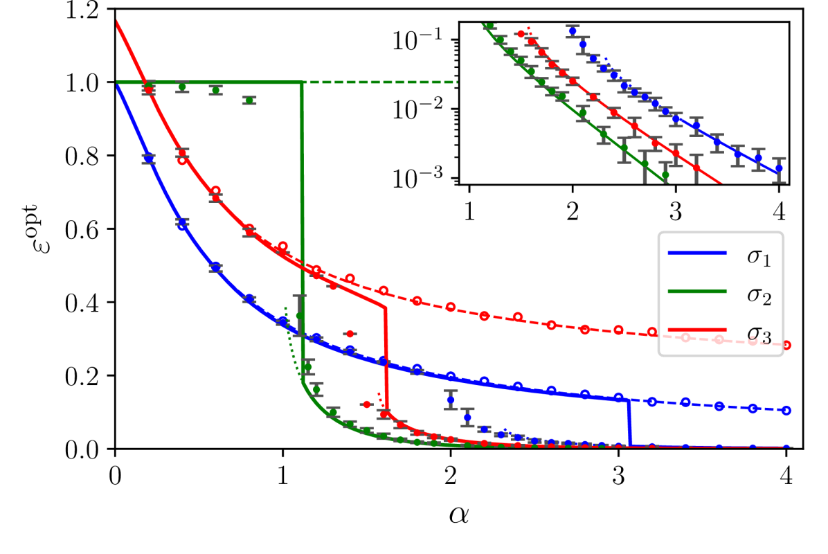
The image presents a chart illustrating the relationship between an optimal error value (εopt) and a parameter alpha (α). The chart uses a logarithmic y-axis and displays three data series, each representing a different sigma value (σ1, σ2, σ3). Error bars are included for each data point, indicating the uncertainty in the measurements.
### Components/Axes
* **X-axis:** Labeled "α" (alpha), ranging from approximately 0 to 4.
* **Y-axis:** Labeled "εopt" (optimal error), using a logarithmic scale ranging from approximately 0.001 to 1.2. The scale is marked with values 10^-3, 10^-2, 10^-1, 1, and 1.2.
* **Legend:** Located in the top-right corner, identifying the three data series:
* σ1 (Blue line)
* σ2 (Green line)
* σ3 (Red line with circle markers)
* **Data Series:** Three lines with associated error bars representing the optimal error for each sigma value.
* **Horizontal dashed line:** A horizontal dashed line at approximately εopt = 1.0.
### Detailed Analysis
**σ1 (Blue Line):**
The blue line representing σ1 starts at approximately εopt = 0.65 when α = 0. It decreases rapidly, approaching εopt = 0.15 at α = 2, and then levels off, reaching approximately εopt = 0.08 at α = 4. The error bars are relatively large at lower alpha values (α < 1) and decrease as alpha increases.
* α = 0, εopt ≈ 0.65, Error ≈ 0.05
* α = 0.5, εopt ≈ 0.4, Error ≈ 0.03
* α = 1, εopt ≈ 0.25, Error ≈ 0.02
* α = 2, εopt ≈ 0.15, Error ≈ 0.01
* α = 3, εopt ≈ 0.09, Error ≈ 0.005
* α = 4, εopt ≈ 0.08, Error ≈ 0.003
**σ2 (Green Line):**
The green line representing σ2 starts at approximately εopt = 1.0 when α = 0. It decreases more steeply than σ1, reaching εopt = 0.1 at α = 1.5, and then levels off, reaching approximately εopt = 0.03 at α = 4. The error bars are also large at lower alpha values and decrease with increasing alpha.
* α = 0, εopt ≈ 1.0, Error ≈ 0.1
* α = 0.5, εopt ≈ 0.6, Error ≈ 0.05
* α = 1, εopt ≈ 0.25, Error ≈ 0.03
* α = 1.5, εopt ≈ 0.1, Error ≈ 0.015
* α = 2, εopt ≈ 0.06, Error ≈ 0.008
* α = 3, εopt ≈ 0.03, Error ≈ 0.003
* α = 4, εopt ≈ 0.02, Error ≈ 0.002
**σ3 (Red Line with Circle Markers):**
The red line representing σ3 starts at approximately εopt = 1.0 when α = 0. It decreases at a rate between σ1 and σ2, reaching εopt = 0.2 at α = 1.5, and then levels off, reaching approximately εopt = 0.05 at α = 4. The error bars are similar in magnitude to σ2.
* α = 0, εopt ≈ 1.0, Error ≈ 0.1
* α = 0.5, εopt ≈ 0.75, Error ≈ 0.06
* α = 1, εopt ≈ 0.4, Error ≈ 0.04
* α = 1.5, εopt ≈ 0.2, Error ≈ 0.02
* α = 2, εopt ≈ 0.12, Error ≈ 0.01
* α = 3, εopt ≈ 0.06, Error ≈ 0.005
* α = 4, εopt ≈ 0.05, Error ≈ 0.004
### Key Observations
* All three data series show a decreasing trend of εopt as α increases.
* σ2 exhibits the steepest decline in εopt with increasing α.
* The error bars indicate greater uncertainty in the measurements at lower values of α.
* All three lines converge towards very low values of εopt as α approaches 4.
* The horizontal dashed line at εopt = 1.0 serves as a reference point, showing that all three curves start above this value and decrease below it.
### Interpretation
The chart demonstrates the relationship between an optimal error (εopt) and a parameter alpha (α) for three different sigma values (σ1, σ2, and σ3). The decreasing trend of εopt with increasing α suggests that as α increases, the optimal error decreases, indicating improved performance or accuracy. The different rates of decline for each sigma value suggest that the optimal error is sensitive to the choice of sigma. The convergence of the lines at higher α values indicates that the effect of sigma becomes less pronounced as α increases. The error bars highlight the uncertainty associated with the measurements, particularly at lower α values, suggesting that the optimal error is more sensitive to variations in the data at lower α values. The horizontal dashed line at εopt = 1.0 provides a baseline for comparison, showing that the optimal error consistently improves as α increases beyond a certain point. This data could be used to optimize a system or algorithm by selecting an appropriate value of α based on the desired level of accuracy and the chosen sigma value.