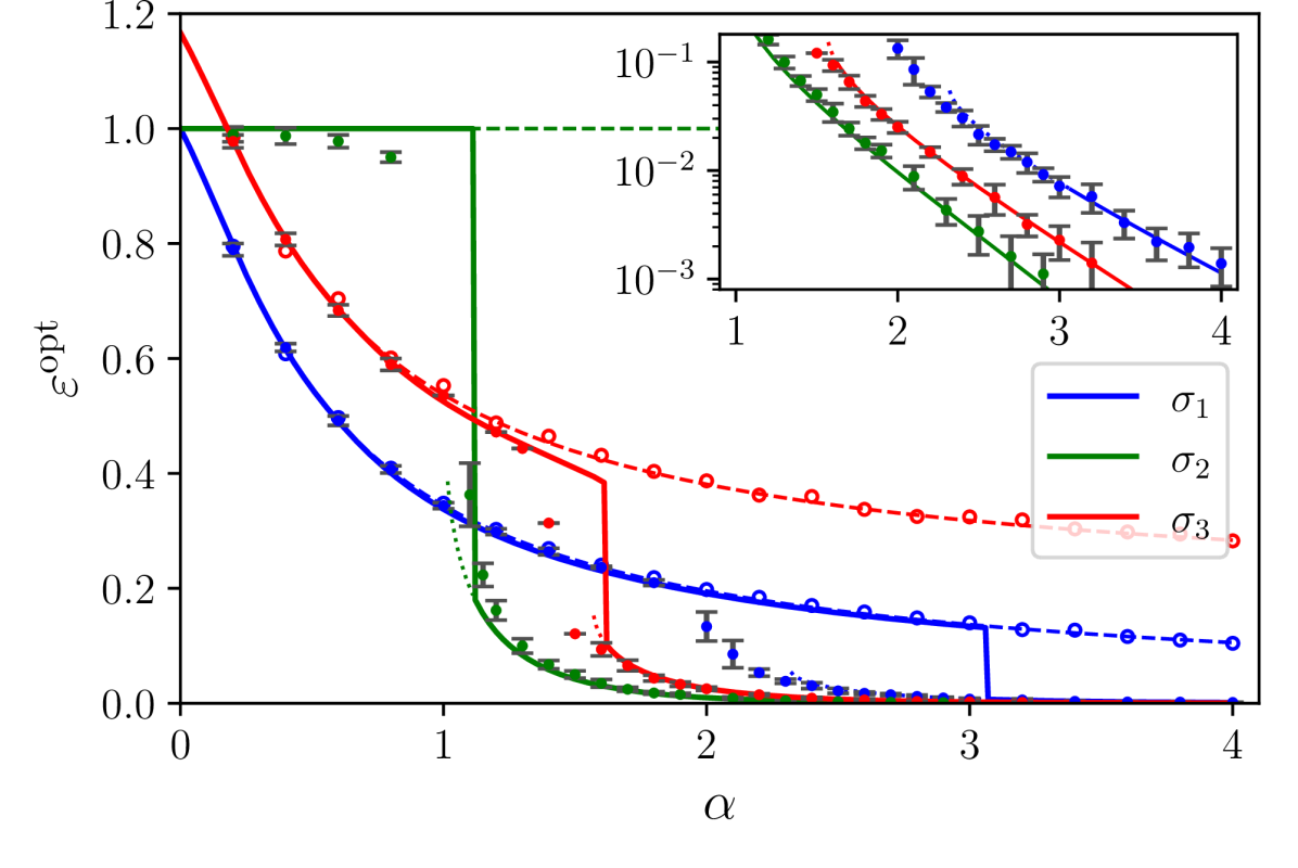
## [Line Graph with Inset]: ε_opt vs. α for Three Series (σ₁, σ₂, σ₃) ### Overview The image is a scientific line graph (with a logarithmic inset) illustrating the relationship between a parameter \( \boldsymbol{\alpha} \) (x-axis) and an optimized quantity \( \boldsymbol{\varepsilon_{\text{opt}}} \) (y-axis). Three data series (\( \sigma_1 \), \( \sigma_2 \), \( \sigma_3 \)) are plotted with error bars, and an inset (top-right) provides a logarithmic view of the same data for small \( \varepsilon_{\text{opt}} \) values. ### Components/Axes #### Main Graph (Linear Scale) - **X-axis**: Label \( \boldsymbol{\alpha} \), range \( 0 \) to \( 4 \) (ticks at \( 0, 1, 2, 3, 4 \)). - **Y-axis**: Label \( \boldsymbol{\varepsilon_{\text{opt}}} \), range \( 0 \) to \( 1.2 \) (ticks at \( 0, 0.2, 0.4, 0.6, 0.8, 1.0, 1.2 \)). - **Legend**: Positioned at the bottom-right (relative to the main graph), with three entries: - Blue line: \( \sigma_1 \) - Green line: \( \sigma_2 \) - Red line: \( \sigma_3 \) #### Inset Graph (Logarithmic Y-axis, Top-Right) - **X-axis**: Range \( 1 \) to \( 4 \) (ticks at \( 1, 2, 3, 4 \)). - **Y-axis**: Logarithmic scale (labels: \( 10^{-3}, 10^{-2}, 10^{-1} \)), showing small \( \varepsilon_{\text{opt}} \) values. - **Data Series**: Same colors (blue, green, red) as the main graph, with error bars. ### Detailed Analysis #### Main Graph (ε_opt vs. α) - **\( \boldsymbol{\sigma_1} \) (Blue Line)**: - Trend: Decreasing with \( \alpha \). At \( \alpha = 0 \), \( \varepsilon_{\text{opt}} \approx 1.0 \); at \( \alpha = 4 \), \( \varepsilon_{\text{opt}} \approx 0.1 \) (dashed line, likely a fit/extrapolation). - Error bars: Present, indicating variability. - **\( \boldsymbol{\sigma_2} \) (Green Line)**: - Trend: Decreasing, with a sharp drop at \( \alpha \approx 1 \) (from \( \approx 1.0 \) to \( \approx 0.2 \)), then continues decreasing. At \( \alpha = 4 \), \( \varepsilon_{\text{opt}} \approx 0.0 \) (or very low). - Error bars: Larger near \( \alpha \approx 1 \) (critical region). - **\( \boldsymbol{\sigma_3} \) (Red Line)**: - Trend: Decreasing, with a sharp drop at \( \alpha \approx 2 \) (from \( \approx 0.4 \) to \( \approx 0.1 \)), then continues decreasing. At \( \alpha = 4 \), \( \varepsilon_{\text{opt}} \approx 0.0 \) (or very low). - Error bars: Larger near \( \alpha \approx 2 \) (critical region). - **Dashed Lines**: For \( \sigma_1 \) (blue) and \( \sigma_3 \) (red), dashed lines extend beyond solid lines (likely model fits/extrapolations). #### Inset Graph (Logarithmic Y-axis) - **\( \boldsymbol{\sigma_1} \) (Blue)**: Decreasing trend. At \( \alpha = 1 \), \( \varepsilon_{\text{opt}} \approx 10^{-1} \); at \( \alpha = 4 \), \( \varepsilon_{\text{opt}} \approx 10^{-3} \). - **\( \boldsymbol{\sigma_2} \) (Green)**: Decreasing trend (steeper than \( \sigma_1 \) in the inset). At \( \alpha = 1 \), \( \varepsilon_{\text{opt}} \approx 10^{-1} \); at \( \alpha = 4 \), \( \varepsilon_{\text{opt}} \approx 10^{-3} \). - **\( \boldsymbol{\sigma_3} \) (Red)**: Decreasing trend. At \( \alpha = 1 \), \( \varepsilon_{\text{opt}} \approx 10^{-1} \); at \( \alpha = 4 \), \( \varepsilon_{\text{opt}} \approx 10^{-3} \). ### Key Observations - **Trends**: All three series show \( \varepsilon_{\text{opt}} \) decreasing with \( \alpha \), but with distinct sharp drops ( \( \sigma_2 \) at \( \alpha \approx 1 \), \( \sigma_3 \) at \( \alpha \approx 2 \)). - **Error Bars**: Larger errors near critical regions (sharp drops), indicating increased variability. - **Inset**: Confirms the decreasing trend for small \( \varepsilon_{\text{opt}} \) values, showing the trend continues beyond the main graph’s visible range. ### Interpretation - The graph likely models an optimization problem where \( \varepsilon_{\text{opt}} \) (e.g., error/efficiency) decreases as \( \alpha \) (a control parameter) increases. Sharp drops suggest **phase transitions** or critical points (e.g., \( \sigma_2 \) transitions at \( \alpha \approx 1 \), \( \sigma_3 \) at \( \alpha \approx 2 \)). - Different series (\( \sigma_1, \sigma_2, \sigma_3 \)) may represent distinct system configurations, showing how optimization behavior varies with conditions. - The inset’s log scale clarifies behavior at small \( \varepsilon_{\text{opt}} \), confirming the trend persists for large \( \alpha \). - Larger error bars near critical regions imply more complex dynamics (e.g., increased uncertainty in measurements or model behavior). (Note: All values are approximate, with uncertainty indicated by error bars. The language is English; no other languages are present.)