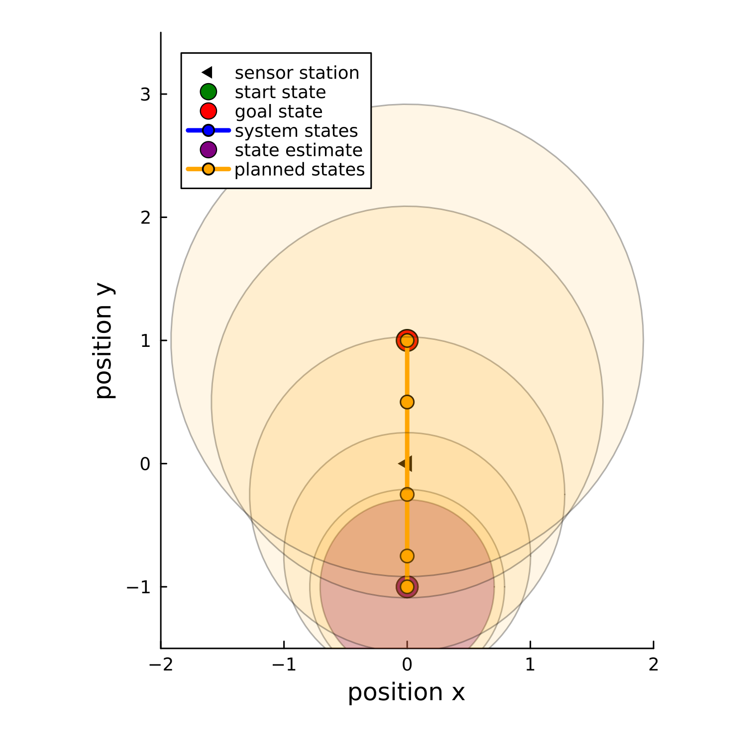
## Diagram: Path Planning and Sensor Range Visualization ### Overview This image is a 2D Cartesian coordinate plot illustrating a path planning scenario. It displays a sensor station at the origin, a state estimate at the bottom, a goal state at the top, and a series of planned states connecting them. Concentric circles centered at the origin likely represent sensor range, uncertainty, or signal strength zones. ### Components/Axes * **X-axis:** Labeled "position x". Range from -2 to 2, with major ticks at -2, -1, 0, 1, 2. * **Y-axis:** Labeled "position y". Range from -1.5 to 3, with major ticks at -1, 0, 1, 2, 3. * **Legend (Top-Left):** * Black triangle: "sensor station" * Green circle: "start state" * Red circle: "goal state" * Blue line with blue circle: "system states" * Purple circle: "state estimate" * Orange line with orange circle: "planned states" ### Detailed Analysis #### 1. Spatial Elements and Positioning * **Sensor Station:** A black triangle is positioned exactly at the origin (0, 0). * **State Estimate:** A purple circle is positioned at (0, -1). * **Goal State:** A red circle is positioned at (0, 1). * **Planned States:** An orange line connects the state estimate (0, -1) to the goal state (0, 1). Along this line, there are intermediate orange circles at approximately: * (0, -0.75) * (0, -0.25) * (0, 0.25) * (0, 0.5) * (0, 0.75) * **Concentric Circles:** Four concentric circles are centered at (0, 0). * **Inner Circle:** Filled with a reddish-brown color, radius approximately 0.75. * **Second Circle:** Filled with light orange, radius approximately 1.25. * **Third Circle:** Filled with very light orange, radius approximately 2.0. * **Outer Circle:** Outlined in faint grey, radius approximately 2.9. #### 2. Trend Verification * **Path Trend:** The "planned states" form a perfectly vertical, linear path along the Y-axis, moving from the state estimate at y = -1 to the goal state at y = 1. * **Uncertainty/Range Trend:** The concentric circles expand outward from the sensor station at (0, 0), suggesting a gradient of influence or uncertainty that increases with distance from the origin. ### Key Observations * **Legend Discrepancy:** There is a notable discrepancy between the legend and the plotted data. The legend includes "start state" (green) and "system states" (blue), but neither green nor blue elements are present in the plot. * **Path Linearity:** The planned path is strictly linear, suggesting a direct movement vector toward the goal, passing directly through the sensor station. * **Visual Hierarchy:** The "goal state" (red) and "state estimate" (purple) are larger than the intermediate "planned states" (orange), emphasizing the start and end points of the trajectory. ### Interpretation This diagram represents a classic robotics or control theory problem: **Path Planning under Sensor Constraints.** * **The Scenario:** An agent (represented by the state estimate) is attempting to navigate from a position at (0, -1) to a goal at (0, 1). * **The Sensor:** The sensor station at (0, 0) is the focal point of the concentric circles. These circles likely represent a "sensor field" or "uncertainty zone." The fact that the path passes directly through the center of these circles suggests the agent is moving through the sensor's field of view or range. * **The Missing Data:** The absence of the "start state" (green) and "system states" (blue) suggests this might be a snapshot of a specific phase of a simulation where only the *estimate* and the *plan* are relevant, or perhaps the "state estimate" has superseded the "start state." * **Peircean Investigative Note:** The concentric circles are not uniform in color; the transition from reddish-brown to light orange suggests a decay in signal quality or an increase in positional uncertainty as the agent moves away from the sensor station. The path is direct, implying that the sensor station is either the target or a waypoint that must be traversed to reach the goal.