## Neural Network Diagram: PDE Approximation ### Overview The image is a diagram illustrating a neural network architecture used to approximate the solution of a partial differential equation (PDE). The diagram shows the flow of information from an input signal, through a neural network, and finally to an output that represents the PDE solution. The network is trained using two loss functions: one based on the data and another based on the PDE itself. ### Components/Axes * **Input:** A visual representation of an input signal, depicted as a wave pattern with sensors. The input is also represented as a set of parameters {s\_m(ω)}\_{m=1}\^M. * **Neural Network:** A multi-layer perceptron (MLP) with input nodes labeled x, y, and z. The network has an intermediate layer represented by an ellipsis (...), and an output node labeled u. * **PDE Operator:** A series of mathematical operations applied to the output of the neural network. These operations include the Laplacian operator (∇²\_r) and the addition of a term k². * **Output:** A visual representation of the output signal, depicted as a wave pattern. * **Loss Functions:** Two loss functions are used to train the network: I\_data and I\_PDE. ### Detailed Analysis or Content Details 1. **Input Signal:** * The input signal is represented by a wave pattern. * Sensors are placed on the wave pattern. * The input is parameterized as {s\_m(ω)}\_{m=1}\^M. 2. **Neural Network:** * The input layer has three nodes labeled x, y, and z. * The network has multiple layers, with an intermediate layer represented by an ellipsis. * The output layer has a single node labeled u. * Connections between layers are represented by arrows. 3. **PDE Operator:** * The output of the neural network (u) is fed into a PDE operator. * The first operation is the Laplacian operator (∇²\_r). * The second operation adds a term k² to the result of the Laplacian operator (∇²\_r + k²). 4. **Output Signal:** * The output signal is represented by a wave pattern. 5. **Loss Functions:** * The loss function I\_data is calculated based on the input signal and the output of the neural network. * The loss function I\_PDE is calculated based on the output of the PDE operator. * Both loss functions are used to train the neural network. ### Key Observations * The diagram illustrates a common approach for solving PDEs using neural networks. * The neural network learns to approximate the solution of the PDE by minimizing the loss functions. * The use of two loss functions (I\_data and I\_PDE) allows the network to learn from both the input data and the PDE itself. ### Interpretation The diagram demonstrates a physics-informed neural network (PINN) approach to solving PDEs. The neural network is trained to approximate the solution of a PDE by minimizing a loss function that includes both data-driven and physics-based terms. The data-driven term (I\_data) encourages the network to fit the available data, while the physics-based term (I\_PDE) enforces the PDE constraint. This approach allows the network to learn the underlying physics of the problem, even when data is sparse or noisy. The input wave pattern and sensor placement suggest a spatial or temporal domain where the PDE is defined. The output wave pattern represents the solution to the PDE that the neural network has learned to approximate.

\n ## Diagram: Physics-Informed Neural Network (PINN) Architecture ### Overview This diagram illustrates the architecture of a Physics-Informed Neural Network (PINN). It depicts the flow of information from an input field, through a neural network, to an output field, incorporating a physics-based loss function. The diagram highlights the data-driven and physics-constrained aspects of the PINN approach. ### Components/Axes The diagram consists of three main sections: Input, Neural Network, and Output. * **Input:** Labeled "{s_m(ω)}^M_m=1", representing a set of data points. The input is visualized as a circular field with concentric wave-like patterns, colored in shades of red and blue. * **Neural Network:** A multi-layered neural network with input nodes labeled 'x', 'y', and 'z', and an output node labeled 'u'. The network has hidden layers represented by interconnected circles. * **Output:** Visualized as a circular field with concentric wave-like patterns, similar to the input, colored in shades of red and blue. * **Loss Functions:** Two loss functions are indicated: "J_data" connected to the input and "J_PDE" connected to the output. * **Physics Constraint:** A box containing the equation "∇²_r∇²_r + k²" represents the physics-based constraint incorporated into the loss function. ### Detailed Analysis or Content Details The input field shows a distribution of data points, represented by small circular markers. These points are likely samples from a physical system. The neural network takes these data points as input and learns to map them to the output field. The output field represents the predicted solution to the underlying physical problem. The physics constraint, ∇²_r∇²_r + k², is used to enforce the governing equations of the physical system. This constraint is incorporated into the loss function (J_PDE), which penalizes deviations from the physics-based model. The neural network architecture appears to be a fully connected feedforward network. The number of layers and nodes in each layer is not explicitly specified, but the diagram shows at least one hidden layer. ### Key Observations * The diagram emphasizes the integration of data and physics in the learning process. * The use of a physics-based loss function allows the PINN to learn solutions that are consistent with the underlying physical laws. * The input and output fields share a similar structure, suggesting that the PINN is learning to reconstruct or extrapolate the input field based on the physics constraint. * The equation within the box is a second-order differential operator, likely representing a wave equation or similar physical model. ### Interpretation This diagram illustrates a powerful approach to solving physical problems using machine learning. PINNs combine the strengths of data-driven modeling and physics-based modeling. By incorporating physical constraints into the learning process, PINNs can achieve higher accuracy and generalization performance than traditional machine learning methods. The diagram suggests that the PINN is being used to solve a problem involving wave propagation or a similar phenomenon described by the given differential equation. The input data likely represents measurements of the physical system, and the output data represents the predicted solution. The physics-based loss function ensures that the predicted solution satisfies the governing equations of the physical system. The use of concentric wave-like patterns in the input and output fields suggests that the problem involves a radially symmetric solution. The parameter 'k' in the physics constraint likely represents a wave number or frequency. The diagram provides a high-level overview of the PINN architecture. Further details about the specific implementation, such as the network architecture, loss function weights, and training procedure, would be needed to fully understand the model.

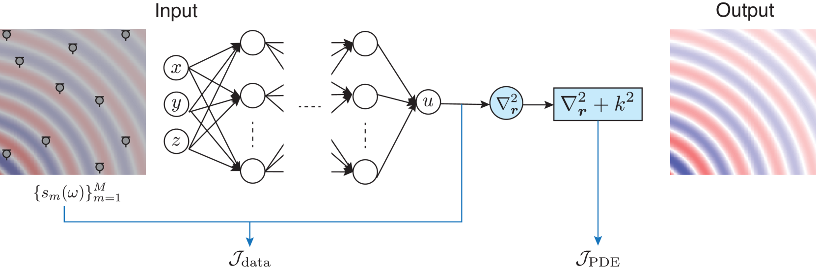
## Diagram: Neural Network Processing with PDE Output ### Overview The diagram illustrates a computational pipeline where input data undergoes transformation through a neural network architecture, followed by a partial differential equation (PDE) operator, to produce an output. The input and output are visualized as heatmaps with radial gradient patterns, while the neural network and PDE components are represented as interconnected nodes and mathematical operators. ### Components/Axes 1. **Input Section**: - **Heatmap**: Labeled "Input" with a radial gradient (blue to red) and scattered black symbols (possibly data points or markers). - **Mathematical Notation**: `{s_m(ω)}^M_{m=1}` indicates a set of M functions or signals parameterized by ω, indexed from m=1 to M. 2. **Neural Network**: - **Nodes**: Labeled `x`, `y`, `z`, and `u` (possibly input, hidden, and output layers). - **Connections**: Dense interconnections between nodes, with dashed lines suggesting optional or residual pathways. - **Data Flow**: Arrows labeled `J_data` indicate the flow of input data through the network. 3. **PDE Operator**: - **Block**: Contains the equation `∇²_r + k²`, where `∇²_r` is the Laplacian operator in radial coordinates and `k²` is a constant term. - **Data Flow**: Arrows labeled `J_PDE` show the output of the neural network being processed by the PDE operator. 4. **Output Section**: - **Heatmap**: Labeled "Output" with a similar radial gradient pattern to the input, suggesting a transformed version of the input data. ### Detailed Analysis - **Input Heatmap**: The radial gradient (blue to red) likely represents a spatial or frequency-domain signal, with black symbols marking specific data points or features. - **Neural Network**: The architecture includes at least three layers (x, y, z) and a final node `u`. The dense connectivity implies a fully connected feedforward network, while dashed lines may indicate skip connections or dropout layers. - **PDE Operator**: The term `∇²_r + k²` suggests a Helmholtz equation or similar PDE, where `k²` acts as a wavenumber squared term. This operator likely models wave propagation or diffusion processes. - **Output Heatmap**: The output pattern mirrors the input's radial structure but with altered intensity, indicating the neural network and PDE have modified the input signal. ### Key Observations 1. **Symmetry in Input/Output**: Both heatmaps exhibit concentric ring patterns, implying the system preserves spatial or frequency-domain structure while modifying amplitude. 2. **PDE Integration**: The explicit inclusion of `∇²_r + k²` suggests the model incorporates physical laws (e.g., wave equations) into the neural network's output. 3. **Data Flow**: The labels `J_data` and `J_PDE` clarify the direction of information processing: input → neural network → PDE → output. ### Interpretation This diagram represents a hybrid model combining machine learning and physics-based modeling. The neural network learns to map input data (e.g., sensor measurements or simulated signals) to an intermediate representation, which is then refined using a PDE to produce a physically consistent output. Applications could include: - **Inverse Problems**: Reconstructing hidden variables (e.g., subsurface structures) from surface measurements. - **Signal Processing**: Enhancing or denoising signals while preserving physical constraints. - **Simulation**: Accelerating PDE-based simulations using learned neural network components. The absence of numerical values or explicit training data suggests this is a conceptual or architectural diagram. The use of radial gradients in input/output heatmaps implies the system is designed for problems with rotational symmetry (e.g., acoustics, electromagnetics, or fluid dynamics).