## Neural Network Diagram: PDE Approximation
### Overview
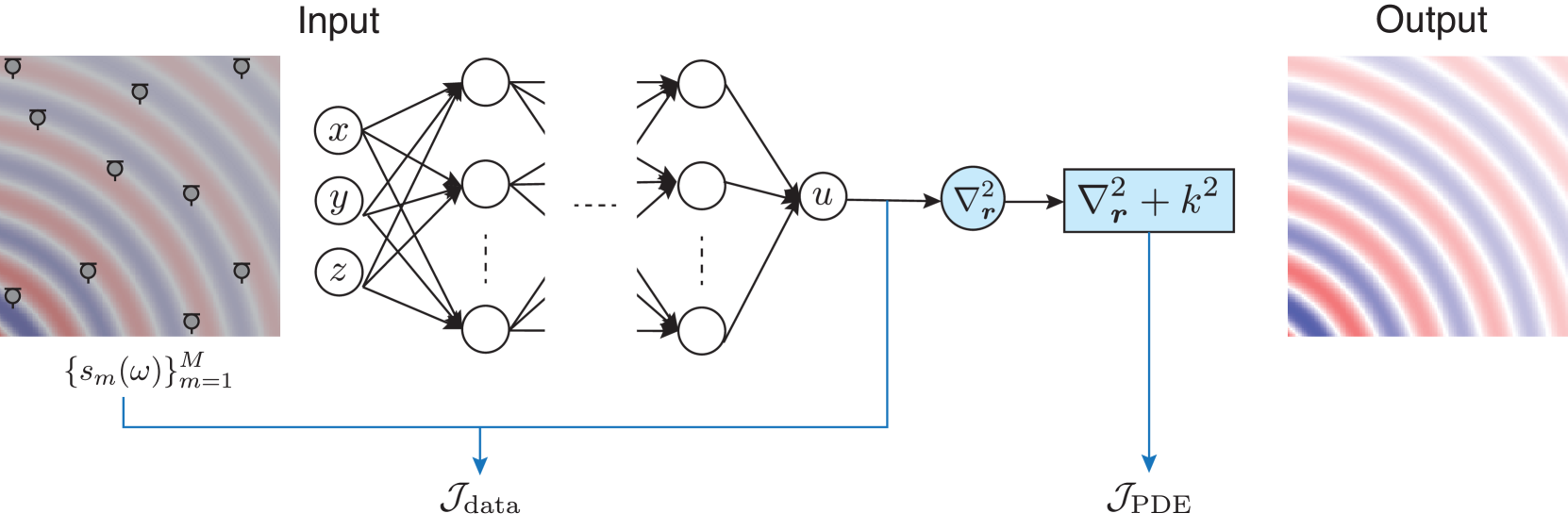
The image is a diagram illustrating a neural network architecture used to approximate the solution of a partial differential equation (PDE). The diagram shows the flow of information from an input signal, through a neural network, and finally to an output that represents the PDE solution. The network is trained using two loss functions: one based on the data and another based on the PDE itself.
### Components/Axes
* **Input:** A visual representation of an input signal, depicted as a wave pattern with sensors. The input is also represented as a set of parameters {s\_m(ω)}\_{m=1}\^M.
* **Neural Network:** A multi-layer perceptron (MLP) with input nodes labeled x, y, and z. The network has an intermediate layer represented by an ellipsis (...), and an output node labeled u.
* **PDE Operator:** A series of mathematical operations applied to the output of the neural network. These operations include the Laplacian operator (∇²\_r) and the addition of a term k².
* **Output:** A visual representation of the output signal, depicted as a wave pattern.
* **Loss Functions:** Two loss functions are used to train the network: I\_data and I\_PDE.
### Detailed Analysis or Content Details
1. **Input Signal:**
* The input signal is represented by a wave pattern.
* Sensors are placed on the wave pattern.
* The input is parameterized as {s\_m(ω)}\_{m=1}\^M.
2. **Neural Network:**
* The input layer has three nodes labeled x, y, and z.
* The network has multiple layers, with an intermediate layer represented by an ellipsis.
* The output layer has a single node labeled u.
* Connections between layers are represented by arrows.
3. **PDE Operator:**
* The output of the neural network (u) is fed into a PDE operator.
* The first operation is the Laplacian operator (∇²\_r).
* The second operation adds a term k² to the result of the Laplacian operator (∇²\_r + k²).
4. **Output Signal:**
* The output signal is represented by a wave pattern.
5. **Loss Functions:**
* The loss function I\_data is calculated based on the input signal and the output of the neural network.
* The loss function I\_PDE is calculated based on the output of the PDE operator.
* Both loss functions are used to train the neural network.
### Key Observations
* The diagram illustrates a common approach for solving PDEs using neural networks.
* The neural network learns to approximate the solution of the PDE by minimizing the loss functions.
* The use of two loss functions (I\_data and I\_PDE) allows the network to learn from both the input data and the PDE itself.
### Interpretation
The diagram demonstrates a physics-informed neural network (PINN) approach to solving PDEs. The neural network is trained to approximate the solution of a PDE by minimizing a loss function that includes both data-driven and physics-based terms. The data-driven term (I\_data) encourages the network to fit the available data, while the physics-based term (I\_PDE) enforces the PDE constraint. This approach allows the network to learn the underlying physics of the problem, even when data is sparse or noisy. The input wave pattern and sensor placement suggest a spatial or temporal domain where the PDE is defined. The output wave pattern represents the solution to the PDE that the neural network has learned to approximate.