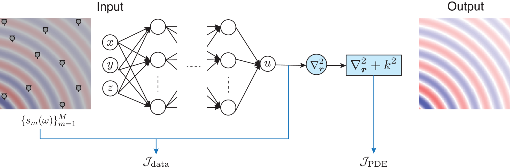
\n ## Diagram: Physics-Informed Neural Network (PINN) Architecture ### Overview This diagram illustrates the architecture of a Physics-Informed Neural Network (PINN). It depicts the flow of information from an input field, through a neural network, to an output field, incorporating a physics-based loss function. The diagram highlights the data-driven and physics-constrained aspects of the PINN approach. ### Components/Axes The diagram consists of three main sections: Input, Neural Network, and Output. * **Input:** Labeled "{s_m(ω)}^M_m=1", representing a set of data points. The input is visualized as a circular field with concentric wave-like patterns, colored in shades of red and blue. * **Neural Network:** A multi-layered neural network with input nodes labeled 'x', 'y', and 'z', and an output node labeled 'u'. The network has hidden layers represented by interconnected circles. * **Output:** Visualized as a circular field with concentric wave-like patterns, similar to the input, colored in shades of red and blue. * **Loss Functions:** Two loss functions are indicated: "J_data" connected to the input and "J_PDE" connected to the output. * **Physics Constraint:** A box containing the equation "∇²_r∇²_r + k²" represents the physics-based constraint incorporated into the loss function. ### Detailed Analysis or Content Details The input field shows a distribution of data points, represented by small circular markers. These points are likely samples from a physical system. The neural network takes these data points as input and learns to map them to the output field. The output field represents the predicted solution to the underlying physical problem. The physics constraint, ∇²_r∇²_r + k², is used to enforce the governing equations of the physical system. This constraint is incorporated into the loss function (J_PDE), which penalizes deviations from the physics-based model. The neural network architecture appears to be a fully connected feedforward network. The number of layers and nodes in each layer is not explicitly specified, but the diagram shows at least one hidden layer. ### Key Observations * The diagram emphasizes the integration of data and physics in the learning process. * The use of a physics-based loss function allows the PINN to learn solutions that are consistent with the underlying physical laws. * The input and output fields share a similar structure, suggesting that the PINN is learning to reconstruct or extrapolate the input field based on the physics constraint. * The equation within the box is a second-order differential operator, likely representing a wave equation or similar physical model. ### Interpretation This diagram illustrates a powerful approach to solving physical problems using machine learning. PINNs combine the strengths of data-driven modeling and physics-based modeling. By incorporating physical constraints into the learning process, PINNs can achieve higher accuracy and generalization performance than traditional machine learning methods. The diagram suggests that the PINN is being used to solve a problem involving wave propagation or a similar phenomenon described by the given differential equation. The input data likely represents measurements of the physical system, and the output data represents the predicted solution. The physics-based loss function ensures that the predicted solution satisfies the governing equations of the physical system. The use of concentric wave-like patterns in the input and output fields suggests that the problem involves a radially symmetric solution. The parameter 'k' in the physics constraint likely represents a wave number or frequency. The diagram provides a high-level overview of the PINN architecture. Further details about the specific implementation, such as the network architecture, loss function weights, and training procedure, would be needed to fully understand the model.