# Technical Data Extraction: OpenWeb Log-Log Plot
## 1. Component Isolation
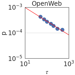
* **Header:** Contains the title "OpenWeb".
* **Main Chart:** A log-log scatter plot with a linear regression line.
* **Axes:**
* **Y-axis (Vertical):** Labeled "$p$", representing a probability or density.
* **X-axis (Horizontal):** Labeled "$\tau$" (tau), representing a time constant or interval.
## 2. Axis Configuration and Scale
The chart utilizes a logarithmic scale (base 10) for both axes, indicating a power-law relationship between the variables.
* **Y-axis ($p$):**
* Range: $10^{-5}$ to $10^{-3}$.
* Major markers: $10^{-5}$, $10^{-4}$, $10^{-3}$.
* A faint horizontal grid line is present at the $10^{-4}$ level.
* **X-axis ($\tau$):**
* Range: $10^1$ (10) to $10^3$ (1000).
* Major markers: $10^1$, $10^3$.
* The midpoint between $10^1$ and $10^3$ (which would be $10^2$ or 100) is not explicitly labeled but is visually the center of the axis.
## 3. Data Series Analysis
### Series 1: Observed Data Points (Blue Circles)
* **Visual Trend:** The data points form a downward-sloping linear pattern on the log-log scale. This confirms a negative power-law correlation.
* **Spatial Distribution:** There are 7 distinct blue circular data points.
* **Estimated Data Points:**
| Point | $\tau$ (approx) | $p$ (approx) |
| :--- | :--- | :--- |
| 1 | $2 \times 10^1$ | $8 \times 10^{-4}$ |
| 2 | $4 \times 10^1$ | $4 \times 10^{-4}$ |
| 3 | $7 \times 10^1$ | $2 \times 10^{-4}$ |
| 4 | $1 \times 10^2$ | $1 \times 10^{-4}$ |
| 5 | $2 \times 10^2$ | $5 \times 10^{-5}$ |
| 6 | $4 \times 10^2$ | $2 \times 10^{-5}$ |
| 7 | $7 \times 10^2$ | $1 \times 10^{-5}$ |
### Series 2: Regression Line (Red Solid Line)
* **Description:** A solid red line passes through the center of the data points, representing the best-fit power-law model.
* **Slope:** The slope is negative, consistent with the decay of $p$ as $\tau$ increases.