## Density Plots: Token Count & Turns (Tool Call)
### Overview
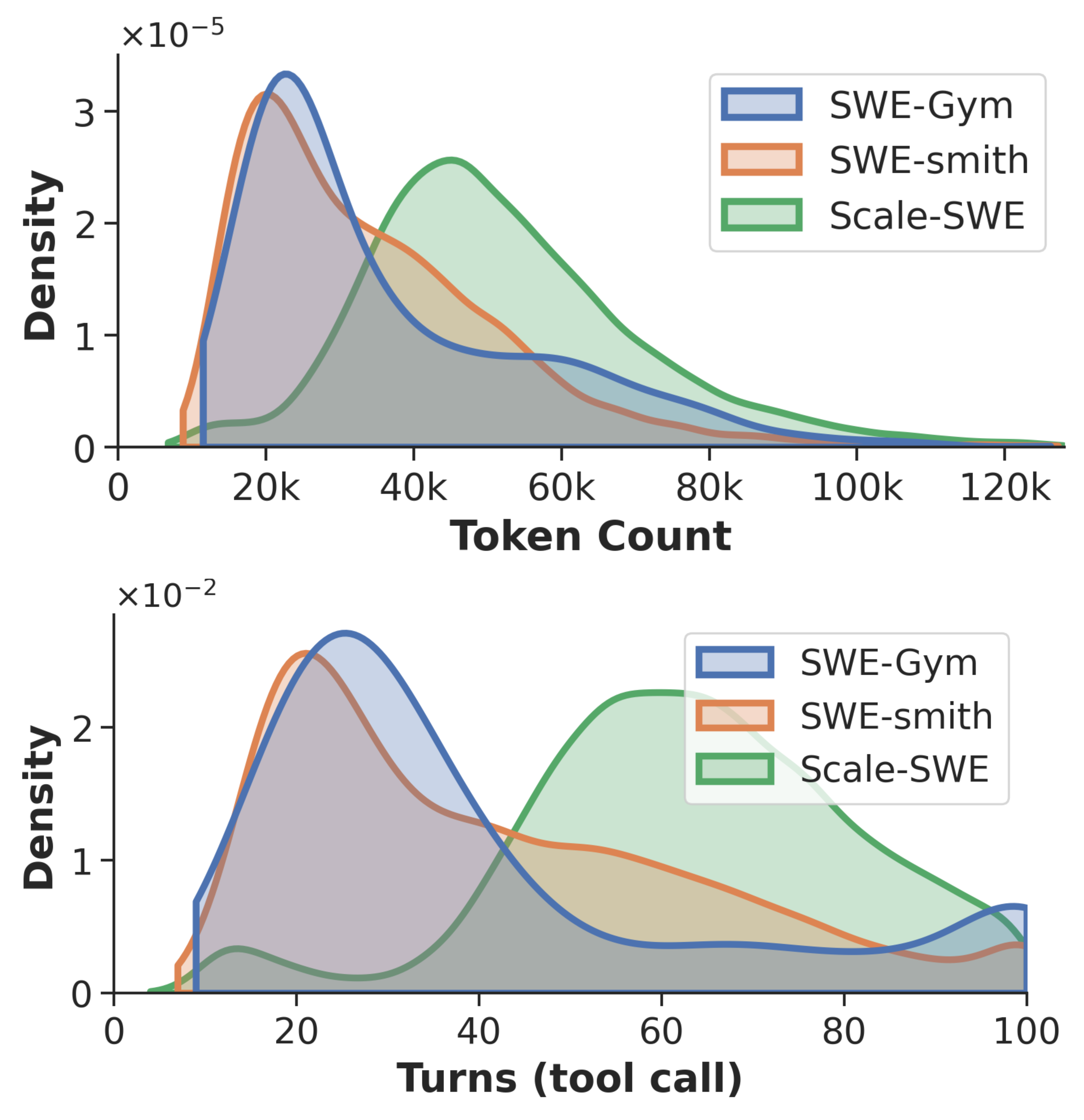
The image presents two density plots, stacked vertically. The top plot visualizes the distribution of "Token Count" for three different models: SWE-Gym, SWE-smith, and Scale-SWE. The bottom plot shows the distribution of "Turns (tool call)" for the same three models. Both plots use density as the y-axis and display the frequency of values along the x-axis.
### Components/Axes
**Top Plot:**
* **X-axis:** "Token Count" ranging from 0 to 120k (120,000), with tick marks at 20k, 40k, 60k, 80k, 100k, and 120k.
* **Y-axis:** "Density" ranging from 0 to approximately 3.2 x 10^-5.
* **Legend (top-right):**
* Blue: SWE-Gym
* Orange: SWE-smith
* Green: Scale-SWE
**Bottom Plot:**
* **X-axis:** "Turns (tool call)" ranging from 0 to 100, with tick marks at 20, 40, 60, 80, and 100.
* **Y-axis:** "Density" ranging from 0 to approximately 2.3 x 10^-2.
* **Legend (top-right):**
* Blue: SWE-Gym
* Orange: SWE-smith
* Green: Scale-SWE
### Detailed Analysis or Content Details
**Top Plot (Token Count):**
* **SWE-Gym (Blue):** The density peaks sharply around 18k-22k tokens. The distribution is heavily skewed to the right, with a long tail extending to approximately 60k tokens, but with very low density beyond that.
* **SWE-smith (Orange):** The density peaks around 28k-32k tokens. The distribution is also skewed to the right, but less so than SWE-Gym. The tail extends further, with some density observed up to 120k tokens, though it is minimal.
* **Scale-SWE (Green):** The density peaks broadly between 35k and 50k tokens. This distribution is the most spread out of the three, with a relatively flat tail extending to 120k tokens.
**Bottom Plot (Turns (tool call)):**
* **SWE-Gym (Blue):** The density peaks sharply around 15-20 turns. The distribution drops off quickly after 30 turns, with very low density beyond 40 turns.
* **SWE-smith (Orange):** The density peaks around 20-25 turns. The distribution is broader than SWE-Gym, with a noticeable density extending to approximately 40-50 turns.
* **Scale-SWE (Green):** The density peaks very weakly around 10-15 turns, and then rises again to a peak around 40-50 turns. This distribution is bimodal, with a significant density between 40 and 80 turns.
### Key Observations
* SWE-Gym generally uses fewer tokens and fewer turns than the other two models.
* Scale-SWE exhibits the widest range of token counts and a bimodal distribution of turns, suggesting more variability in its behavior.
* SWE-smith falls between SWE-Gym and Scale-SWE in terms of both token count and turns.
* The distributions for both Token Count and Turns are right-skewed for SWE-Gym and SWE-smith, indicating that a small number of instances require significantly more tokens/turns.
### Interpretation
These density plots likely represent the performance characteristics of three different language models (SWE-Gym, SWE-smith, and Scale-SWE) on a specific task. The "Token Count" plot indicates the length of the input/output sequences processed by each model, while the "Turns (tool call)" plot indicates the number of interactions required to complete the task.
The data suggests that SWE-Gym is the most efficient model in terms of both token usage and the number of turns required. However, Scale-SWE demonstrates greater variability, potentially indicating a more complex or adaptable behavior. The bimodal distribution of turns for Scale-SWE could suggest that it sometimes requires a significantly different approach to solve the task, leading to a second peak in the distribution.
The differences in distributions could be due to variations in model architecture, training data, or the specific task being performed. Further investigation would be needed to determine the underlying causes of these differences and to assess the trade-offs between efficiency and adaptability. The right skewness in the token count suggests that some inputs require significantly more processing than others, which could be a point of optimization.