# Technical Diagram Analysis: Low-Rank Adaptation (LoRA) Architecture
This document provides a detailed technical extraction of the provided architectural diagram, which illustrates the mathematical flow of a Low-Rank Adaptation (LoRA) module in a neural network.
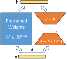
## 1. Component Isolation
The diagram is structured into three vertical layers representing the flow of data from input to output.
### Header (Output Layer)
- **Label:** `h`
- **Component:** A horizontal yellow rectangular bar representing the output vector.
- **Operation:** A plus sign (`+`) is positioned between two upward-pointing arrows, indicating the summation of the outputs from the two parallel paths below.
### Main Body (Processing Layer)
This section contains two parallel paths:
1. **Left Path (Pretrained Weights):**
* **Visual:** A large blue square.
* **Text Label:** "Pretrained Weights"
* **Mathematical Notation:** $W \in \mathbb{R}^{d \times d}$
* **Function:** Represents the frozen, original weight matrix of the model.
2. **Right Path (Low-Rank Adaptation):**
* **Visual:** Two orange trapezoids forming a "bottleneck" shape.
* **Top Trapezoid Label:** $B = 0$ (Indicates the matrix $B$ is initialized to zero).
* **Bottom Trapezoid Label:** $A = \mathcal{N}(0, \sigma^2)$ (Indicates the matrix $A$ is initialized with a Gaussian/Normal distribution).
* **Dimension Label (Middle):** A bracket labeled `r` spans the narrowest part of the bottleneck, representing the low-rank dimension.
### Footer (Input Layer)
- **Label:** `x`
- **Component:** A horizontal yellow rectangular bar representing the input vector.
- **Dimension Label:** A bracket labeled `d` spans the width of the input bar, indicating the input dimensionality.
---
## 2. Data Flow and Logic Extraction
The diagram describes the following computational process:
1. **Input Distribution:** The input vector `x` (of dimension `d`) is fed simultaneously into two parallel branches.
2. **Parallel Computation:**
* **Path A (Frozen):** The input is multiplied by the pretrained weight matrix $W$. Because $W$ is "Pretrained," it is typically kept frozen during this specific adaptation process.
* **Path B (Trainable):** The input passes through a low-rank decomposition consisting of two matrices, $A$ and $B$.
* The data first passes through matrix $A$ (reducing dimension from $d$ to $r$).
* The data then passes through matrix $B$ (increasing dimension from $r$ back to $d$).
3. **Initialization State:**
* Matrix $A$ is initialized using a random normal distribution: $\mathcal{N}(0, \sigma^2)$.
* Matrix $B$ is initialized as a zero matrix ($B = 0$), ensuring that at the start of training, the entire LoRA side-path contributes nothing to the output, making the initial output identical to the original pretrained model.
4. **Recombination:** The results from the pretrained weights and the low-rank adaptation path are added together (indicated by the `+` symbol) to produce the final output `h`.
---
## 3. Summary of Mathematical Entities
| Entity | Description | Properties / Initialization |
| :--- | :--- | :--- |
| **x** | Input Vector | Dimension $d$ |
| **W** | Pretrained Weight Matrix | $W \in \mathbb{R}^{d \times d}$ |
| **A** | Down-projection Matrix | Initialized via $\mathcal{N}(0, \sigma^2)$; Rank $r$ |
| **B** | Up-projection Matrix | Initialized to $0$; Rank $r$ |
| **r** | Low-rank Dimension | $r \ll d$ |
| **h** | Output Vector | $h = Wx + BAx$ |