## Diagram: Variational Router Process ### Overview The image illustrates a process flow diagram for a variational router, detailing the steps from input to parameter update. It includes a visual representation of a probability distribution and the sampling methods used during training and inference. ### Components/Axes * **Hidden Token Input:** Labeled as "Hidden Token Input u" in a dashed box. * **Variational Router:** A block labeled "Variational Router" with sub-components: "NNdet(·)", "Δμϕ(·)", and "log σϕ(·)". * **Probability Distribution:** A 3D wireframe plot representing a probability distribution, labeled with "μpost" at the peak and "Σpost" indicating the spread. A blue dot is present on the surface of the distribution. * **Sampling Blocks:** Two blocks representing sampling methods: "Sample once s = softmax(I°)" and "Sample S times s = (1/S) Σ softmax(I°)", where the summation is from s=1 to S. * **Top-K:** A block labeled "Top-K". * **Parameter Update:** A block labeled "Training: Parameter Update" with the equations "LVR = Ltask + β · LKL" and "ϕ ← ϕ - η∇ϕLVR". * **Arrows:** Arrows indicate the flow of information between the components. * **Training/Inference Labels:** Arrows pointing from the probability distribution to the sampling blocks are labeled "Training" and "Inference". ### Detailed Analysis 1. **Input:** The process begins with a "Hidden Token Input u". 2. **Variational Router:** The input is fed into a "Variational Router" which consists of neural network components. 3. **Probability Distribution:** The output of the router is represented as a probability distribution. The peak of the distribution is labeled μpost, and the spread is labeled Σpost. 4. **Sampling:** * **Training:** During training, a sample is drawn once using the softmax function: s = softmax(I°). * **Inference:** During inference, S samples are drawn and averaged: s = (1/S) Σ softmax(I°), where the summation is from s=1 to S. 5. **Top-K:** The samples are then processed by a "Top-K" selection. 6. **Parameter Update:** Finally, the parameters are updated based on the loss function LVR, which is a combination of Ltask and LKL, weighted by β. The update rule is given by ϕ ← ϕ - η∇ϕLVR. ### Key Observations * The diagram illustrates the flow of information and processes within a variational router framework. * It highlights the difference in sampling strategies between training and inference. * The parameter update step involves a loss function that combines task-specific loss and a KL divergence term. ### Interpretation The diagram describes a variational router, a component likely used in a machine learning model. The router takes an input, transforms it into a probability distribution, and then samples from this distribution. The difference in sampling between training and inference suggests a method to improve the model's generalization or exploration capabilities. The parameter update step indicates that the model is being trained to minimize a combination of task-specific loss and a regularization term (KL divergence), which is common in variational inference methods. The blue dot on the probability distribution is likely a visual aid to highlight a specific point or region of interest on the distribution surface.

\n ## Diagram: Variational Router Architecture ### Overview The image depicts a diagram of a Variational Router architecture, illustrating the flow of information from a Hidden Token Input through a Variational Router, a posterior distribution, sampling processes (during training and inference), and finally to a Top-K parameter update stage. The diagram highlights the mathematical operations involved in each step. ### Components/Axes The diagram consists of the following components, arranged from left to right: 1. **Hidden Token Input (u):** The initial input to the system. 2. **Variational Router:** A neural network (NN) that takes the input 'u' and outputs Δμ(⋅), log σ(⋅). 3. **Posterior Distribution:** Represented as a 3D Gaussian surface, labeled with Σ_post and μ_post. 4. **Training Branch:** Indicates sampling once using s = softmax(Γ'). 5. **Inference Branch:** Indicates sampling 's' times using s = Σ_s=1^s softmax(Γ'). 6. **Top-K:** A component for parameter update. 7. **Training Loss:** A box containing the equations for the loss function and parameter update. ### Detailed Analysis or Content Details * **Hidden Token Input (u):** Labeled simply as "Hidden Token Input u". * **Variational Router:** The router is described as NN_φ(⋅), with outputs Δμ(⋅) and log σ(⋅). The φ likely represents the parameters of the neural network. * **Posterior Distribution:** The posterior distribution is characterized by Σ_post (covariance matrix) and μ_post (mean vector). The 3D surface visually represents a Gaussian distribution. * **Training Branch:** The training branch involves sampling once, where 's' is calculated as softmax(Γ'). Γ' is not further defined. * **Inference Branch:** The inference branch involves sampling 's' times, where 's' is calculated as the sum of softmax(Γ') from s=1 to s. * **Top-K:** This component is labeled "Top-K Parameter Update". * **Training Loss:** The training loss is defined by the following equations: * L_VR = L_data + λ L_KL * φ ← φ - η ∇_φL_VR Where: * L_VR is the Variational Router loss. * L_data is the data loss. * L_KL is the KL divergence loss. * λ is a weighting factor. * φ represents the parameters of the network. * η is the learning rate. * ∇_φL_VR is the gradient of the loss with respect to the parameters. ### Key Observations The diagram illustrates a variational inference approach. The Variational Router aims to approximate the posterior distribution. The training process involves minimizing a loss function that balances data fit (L_data) and the KL divergence between the approximate posterior and the true posterior (L_KL). The Top-K component suggests a method for selecting the most important parameters for updating. ### Interpretation This diagram represents a novel approach to routing information within a neural network using variational inference. The Variational Router learns a posterior distribution over possible routes, allowing for more flexible and robust information flow. The use of a variational approach introduces uncertainty into the routing process, which can be beneficial for generalization and exploration. The Top-K parameter update suggests a method for focusing on the most important parameters during training, potentially improving efficiency and performance. The diagram highlights the mathematical foundations of the architecture, emphasizing the use of Gaussian distributions, softmax functions, and gradient-based optimization. The separation of training and inference branches indicates different sampling strategies are employed in each phase. The overall architecture appears designed to address challenges in complex neural networks where traditional routing methods may be insufficient.

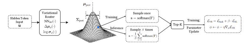
## Technical Diagram: Variational Router Training and Inference Flowchart ### Overview The image is a technical flowchart illustrating a machine learning process involving a "Variational Router" component. It depicts the flow from an input token through a variational distribution, branching into separate training and inference pathways, and culminating in a parameter update step. The diagram is monochrome (black and white) and uses a combination of text boxes, arrows, mathematical notation, and a 3D surface plot to represent the process. ### Components/Axes The diagram is organized horizontally from left to right, with a central 3D plot. The components are: 1. **Input (Far Left):** A dashed box labeled `Hidden Token Input (t)`. 2. **Variational Router (Left-Center):** A solid box labeled `Variational Router`. Inside, three functions are listed vertically: - `SNN(·)` - `Δμ(·)` - `log σ(·)` 3. **Posterior Distribution (Center):** A 3D wireframe surface plot of a bell-shaped (Gaussian) distribution. It is annotated with: - `μ_post` (pointing to the peak along the vertical axis). - `Σ_post` (pointing to the spread/width of the distribution). - A blue dot is placed on the surface of the plot. 4. **Process Branches (Center-Right):** Two parallel paths diverge from the distribution plot: - **Top Path (Training):** Labeled `Training`. Contains a dashed box with the text `Sample once` and the equation `s = softmax(V)`. - **Bottom Path (Inference):** Labeled `Inference`. Contains a dashed box with the text `Sample N times` and the equation `s = 1/N Σ_{i=1}^{N} softmax(V_i)`. 5. **Selection Module (Right-Center):** A solid box labeled `Top-K` that receives input from both the Training and Inference branches. 6. **Parameter Update (Far Right):** A dashed box connected to the `Top-K` module, labeled `Training`. It contains two lines of mathematical text: - `L_VR = L_CE + β · L_KL` - `θ ← θ - α∇_θ L_VR` ### Detailed Analysis - **Flow Direction:** The process flows unidirectionally from left (`Hidden Token Input`) to right (`Parameter Update`). The central distribution acts as a hub, feeding into two distinct operational modes (Training and Inference) which later converge at the `Top-K` module. - **Mathematical Content:** - The Variational Router outputs parameters for a distribution, likely a Gaussian, given `μ_post` (mean) and `Σ_post` (covariance). - The **Training** path uses a single sample (`Sample once`) passed through a softmax function to produce `s`. - The **Inference** path uses an average over `N` samples (`Sample N times`), each passed through softmax, to produce a more stable estimate `s`. - The final loss function `L_VR` is a weighted sum of a Cross-Entropy loss (`L_CE`) and a Kullback-Leibler divergence loss (`L_KL`), scaled by a hyperparameter `β`. - Parameters `θ` are updated via gradient descent with learning rate `α`, using the gradient of the total loss `∇_θ L_VR`. - **Spatial Grounding:** The legend/labels (`Training`, `Inference`) are placed directly above their respective process boxes. The mathematical equations are contained within dashed boxes associated with their respective process step. The 3D plot is centrally located, visually emphasizing its role as the core probabilistic model. ### Key Observations 1. **Dual-Path Architecture:** The system explicitly separates the stochastic sampling process during training (single sample) from the inference phase (averaged over N samples). This is a common technique to balance training efficiency with inference robustness. 2. **Top-K Integration:** Both pathways feed into a `Top-K` module before the final training step. This suggests a selection or filtering mechanism is applied to the outputs (`s`) from either path before computing the loss. 3. **Loss Composition:** The training objective combines a task-specific loss (`L_CE`) with a regularization term (`L_KL`), which is characteristic of variational methods to prevent overfitting and encourage the learned distribution to stay close to a prior. 4. **Visual Emphasis:** The 3D Gaussian plot is the most visually complex element, highlighting the importance of the variational posterior distribution in this architecture. ### Interpretation This diagram outlines a **variational inference framework for a routing mechanism** within a neural network. The "Variational Router" likely decides how to process or route the input token `t` by sampling from a learned probability distribution (`μ_post`, `Σ_post`). - **Purpose:** The system aims to learn a robust routing policy. During training, it uses a noisy, single-sample estimate to explore options. During inference, it uses a smoothed, averaged estimate for stable, reliable decisions. - **Relationships:** The `Top-K` module acts as a bottleneck or selector, possibly choosing the most promising routing decisions before they are used to compute the final loss and update the router's parameters (`θ`). The KL divergence term ensures the learned distribution doesn't deviate too far from a predefined prior, providing regularization. - **Underlying Principle:** This is a **reparameterized gradient estimation** setup (implied by the sampling and backpropagation through `θ`). The architecture is designed to train a stochastic, probabilistic component (the router) within a larger deterministic system using standard gradient-based optimization. The separation of training and inference sampling strategies is a key design choice to mitigate the variance often associated with stochastic units during training.

## Diagram: Variational Router Architecture for Token Sampling ### Overview This diagram illustrates a variational router architecture used in natural language processing (NLP) for token selection. It shows the flow from hidden token input to parameterized distributions, training/inference processes, and parameter updates. The architecture combines probabilistic modeling with optimization techniques to balance exploration and exploitation in token sampling. ### Components/Axes 1. **Input**: - "Hidden Token Input u" (dashed box on the left) 2. **Variational Router**: - Outputs three parameters: - `NN_det(·)` (deterministic neural network) - `Δμ_φ(·)` (mean shift) - `log σ_φ(·)` (log variance) 3. **Gaussian Distribution**: - Visualized as a 3D surface plot - Labeled with: - `μ_post` (posterior mean) - `Σ_post` (posterior covariance) 4. **Training Path**: - "Sample once" block with `s = softmax(l^s)` - "Top-K" selection - Loss function: `L_VR = L_task + β·L_KL` - Parameter update: `φ ← φ - η∇_φL_VR` 5. **Inference Path**: - Two sampling strategies: - Single sample: `s = softmax(l^s)` - Multiple samples: `s = 1/S ∑_{s=1}^S softmax(l^s)` ### Detailed Analysis - **Gaussian Distribution**: The 3D plot shows a unimodal distribution centered at `μ_post` with spread determined by `Σ_post`. The dashed lines indicate confidence intervals around the mean. - **Training Process**: - Uses softmax to convert logits `l^s` into probabilities - Applies Top-K sampling to select most probable tokens - Combines task loss (`L_task`) with KL divergence (`L_KL`) regularization - Updates parameters using gradient descent with learning rate η - **Inference Process**: - Offers two sampling approaches: 1. Deterministic single-sample softmax 2. Stochastic ensemble sampling (average of S softmax outputs) - **Parameterization**: The variational router parameterizes the posterior distribution through neural network outputs, enabling end-to-end learning of uncertainty estimates. ### Key Observations 1. The architecture explicitly models uncertainty through the variational distribution (μ_post, Σ_post) 2. Training balances task performance (L_task) with distribution fidelity (L_KL) via the β hyperparameter 3. Inference provides flexibility between deterministic and stochastic sampling strategies 4. Top-K sampling introduces a trade-off between exploration (full softmax) and efficiency (limited candidates) ### Interpretation This architecture demonstrates a Bayesian approach to sequence modeling where: - The variational router learns to estimate token uncertainty through posterior distributions - The KL divergence term prevents overconfidence in predictions - The dual sampling strategies in inference allow adaptation to different deployment requirements - The parameter update rule shows standard stochastic gradient descent with backpropagation through the variational objective The diagram reveals a sophisticated method for handling discrete token selection with continuous uncertainty estimation, combining elements of variational inference and neural network training. The use of both single and ensemble sampling in inference suggests an awareness of the exploration-exploitation tradeoff in language generation tasks.