## Diagram: Comparison of Tactic Selection Methods (Conventional vs. TrialMaster)
### Overview
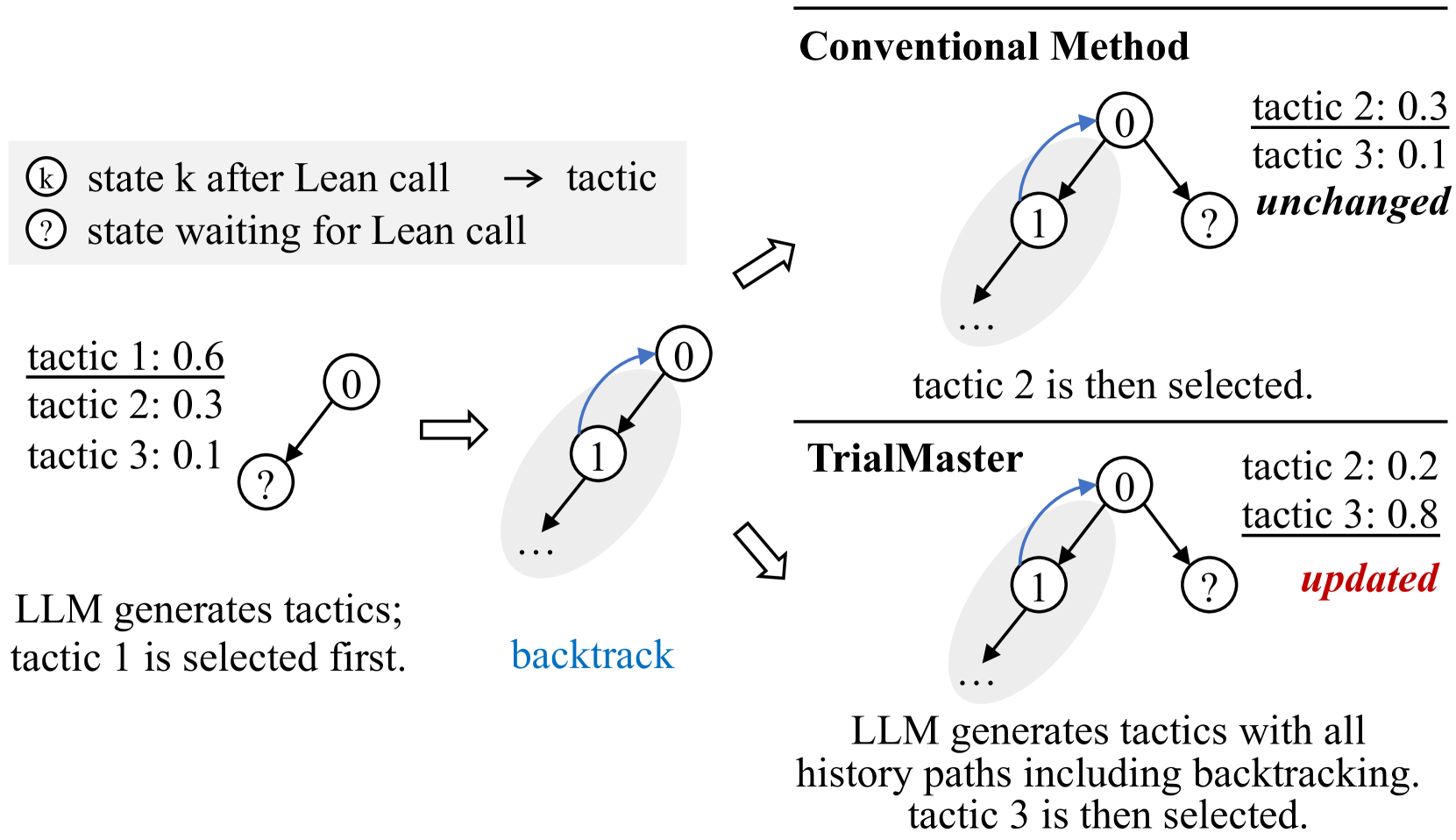
The image is a technical diagram illustrating and comparing two methods for selecting tactics in a system that interacts with a "Lean call" (likely a reference to the Lean theorem prover). It contrasts a "Conventional Method" with a method called "TrialMaster," focusing on how they handle tactic probabilities after a backtracking event. The diagram uses a state-transition graph with nodes and arrows to represent the process flow.
### Components/Axes
**Legend (Top-Left):**
* **Symbol `k` inside a circle:** "state k after Lean call"
* **Symbol `?` inside a circle:** "state waiting for Lean call"
* **Arrow `→`:** "tactic" (indicating a transition labeled with a tactic)
**Main Diagram Structure:**
The diagram is divided into three main sections:
1. **Left Section (Initial State):** Shows the starting point before any method is applied.
2. **Top-Right Section (Conventional Method):** Shows the outcome using the conventional approach.
3. **Bottom-Right Section (TrialMaster):** Shows the outcome using the TrialMaster approach.
**Visual Elements:**
* **Nodes:** Circles containing either a number (e.g., `0`, `1`) or a question mark `?`.
* **Arrows:** Directed lines connecting nodes, representing state transitions. Some arrows are blue.
* **Shaded Ovals:** Gray ellipses grouping certain nodes and transitions, indicating a sub-process or focus area.
* **Text Annotations:** Probabilities, labels, and descriptive sentences placed near the graphical elements.
### Detailed Analysis
**1. Initial State (Left Section):**
* A starting node `0` (state 0 after a Lean call) has an outgoing arrow to a node `?` (state waiting for a Lean call).
* **Associated Text:**
* `tactic 1: 0.6`
* `tactic 2: 0.3`
* `tactic 3: 0.1`
* **Descriptive Text:** "LLM generates tactics; tactic 1 is selected first."
* **Flow:** An arrow points from this initial setup to the next stage, labeled with the blue text "**backtrack**". This indicates that the first selected tactic (tactic 1) led to a need to backtrack.
**2. Backtrack Stage (Center):**
* The diagram shows a node `0` with a blue arrow pointing to a node `1`. Node `1` is inside a gray shaded oval that also contains an outgoing arrow leading to "..." (ellipsis, indicating continuation).
* This represents the state after backtracking from the failed attempt with tactic 1. The system is now at state `1`.
**3. Conventional Method (Top-Right):**
* **Flow:** From the backtrack stage (state `1`), the process continues. The diagram shows node `0` (the original state) with two outgoing arrows:
* One blue arrow to node `1` (the backtracked path).
* One black arrow to a new node `?`.
* **Associated Text (next to the new `?` node):**
* `tactic 2: 0.3`
* `tactic 3: 0.1`
* The word "**unchanged**" is written in bold italics below these probabilities.
* **Descriptive Text:** "tactic 2 is then selected."
* **Interpretation:** The conventional method does not update the probabilities of the remaining tactics (tactic 2 and tactic 3) after the backtracking event. Their probabilities remain at the initial values (0.3 and 0.1, respectively). Tactic 2, having the highest remaining probability, is selected next.
**4. TrialMaster (Bottom-Right):**
* **Flow:** Identical graphical structure to the Conventional Method branch: node `0` with a blue arrow to node `1` and a black arrow to a new node `?`.
* **Associated Text (next to the new `?` node):**
* `tactic 2: 0.2`
* `tactic 3: 0.8`
* The word "**updated**" is written in bold, red italics below these probabilities.
* **Descriptive Text:** "LLM generates tactics with all history paths including backtracking. tactic 3 is then selected."
* **Interpretation:** The TrialMaster method updates the tactic probabilities after incorporating the history of the backtracking event. The probability for tactic 2 decreases from 0.3 to 0.2, while the probability for tactic 3 increases significantly from 0.1 to 0.8. Consequently, tactic 3, now having the highest probability, is selected next.
### Key Observations
1. **Probability Update Mechanism:** The core difference between the two methods is the dynamic updating of tactic probabilities. The Conventional Method uses static probabilities, while TrialMaster adjusts them based on execution history (including failures/backtracks).
2. **Dramatic Probability Shift:** In the TrialMaster example, the probability of tactic 3 increases eightfold (from 0.1 to 0.8) after the backtrack, making it the dominant choice. This suggests the system learned that tactic 1 failed and tactic 2 might be less promising, thereby boosting the relative likelihood of tactic 3.
3. **Visual Consistency:** The graphical structure (nodes, arrows, shaded ovals) is identical for both methods in the right-hand sections, emphasizing that the difference is purely in the associated probability values and the selection logic.
4. **Color Coding:** Blue is used for the "backtrack" label and the arrow representing the backtracking path. Red is used exclusively for the word "updated" in the TrialMaster section, highlighting the key action of that method.
### Interpretation
This diagram illustrates a conceptual improvement in automated reasoning or proof-search systems. The "Conventional Method" represents a naive or memoryless approach where each decision is made based on initial, fixed probabilities, ignoring the outcome of previous attempts. This can lead to inefficient repetition of less promising paths.
**TrialMaster** proposes a more adaptive, history-aware strategy. By updating tactic probabilities based on the success or failure (backtracking) of previous choices, it mimics a form of reinforcement learning. The system "remembers" that tactic 1 led to a dead end and recalibrates its strategy, significantly increasing the probability assigned to tactic 3. This likely leads to more efficient exploration of the search space, avoiding repeated failures and focusing on potentially more fruitful tactics.
The diagram serves as a high-level, intuitive explanation of how incorporating historical context (specifically, backtracking information) into the decision-making process of a Large Language Model (LLM) can lead to different and presumably better tactic selection outcomes. The specific numerical values (0.6, 0.3, 0.1 → 0.2, 0.8) are illustrative examples of this updating mechanism in action.