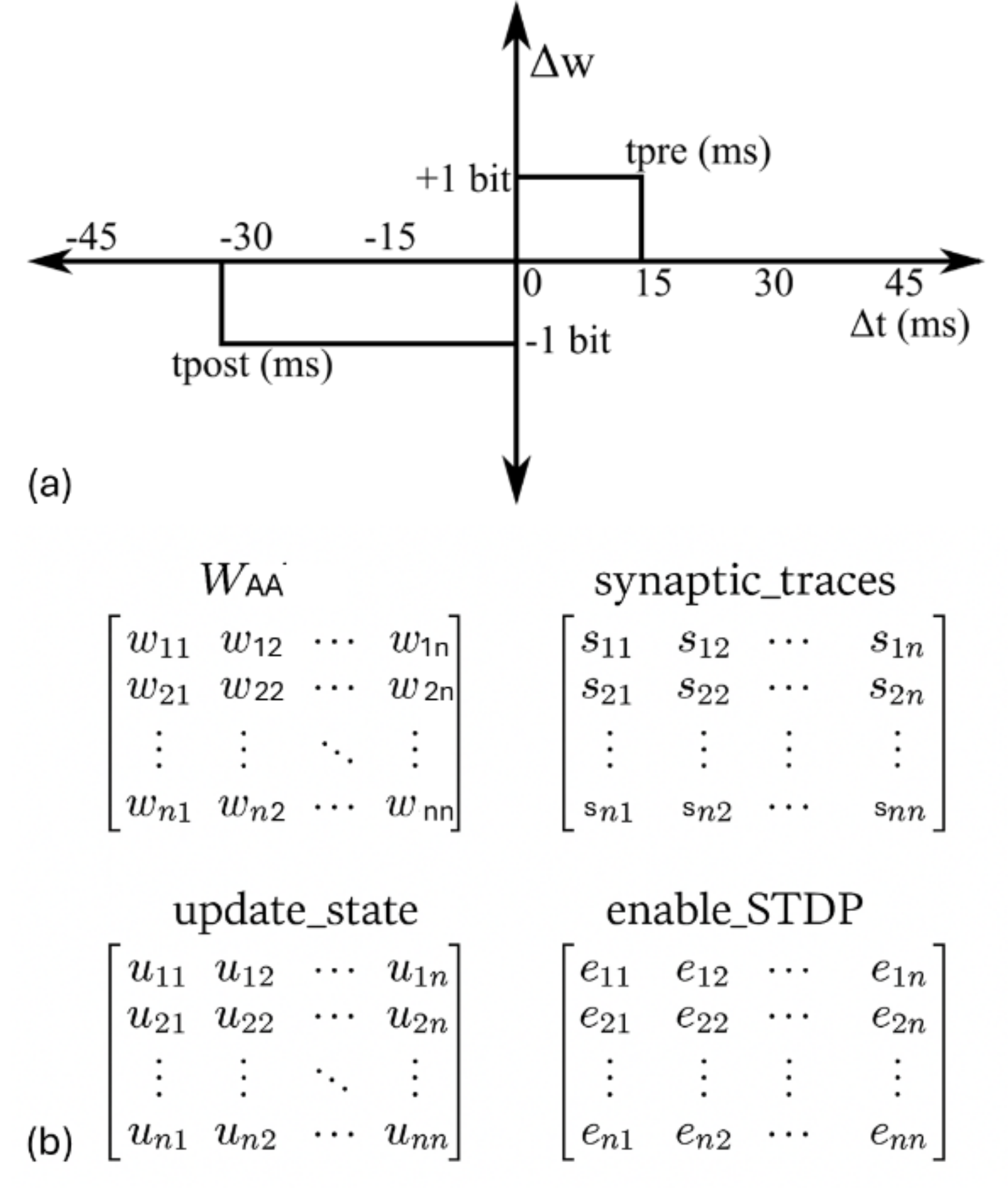
## Technical Diagram: Spike-Timing-Dependent Plasticity (STDP) Rule and Associated Matrices ### Overview The image is a two-part technical diagram illustrating a simplified, binary model of Spike-Timing-Dependent Plasticity (STDP) and the matrix representations of its associated variables in a neural network context. Part (a) is a graph defining the weight update rule based on spike timing differences. Part (b) displays four generic matrices representing the state variables of a network implementing this rule. ### Components/Axes #### Part (a): STDP Rule Graph * **Vertical Axis (Y-axis):** Labeled **Δw**. Represents the change in synaptic weight. The axis has two discrete levels marked: **+1 bit** (positive change) and **-1 bit** (negative change). * **Horizontal Axis (X-axis):** Labeled **Δt (ms)**. Represents the time difference between pre-synaptic and post-synaptic spikes in milliseconds. The axis has tick marks at **-45, -30, -15, 0, 15, 30, 45**. * **Regions and Labels:** * A rectangular region in the positive quadrant (Δt > 0, Δw = +1 bit) is labeled **tpre (ms)**. This region spans from Δt = 0 to Δt = 15 ms. * A rectangular region in the negative quadrant (Δt < 0, Δw = -1 bit) is labeled **tpost (ms)**. This region spans from Δt = -30 ms to Δt = 0. * **Sub-label:** The graph is labeled **(a)** in the bottom-left corner. #### Part (b): Matrix Representations Four matrices are presented, all sharing an identical n x n structure with elements indexed from 1 to n. Ellipses (`...`) indicate the continuation of rows and columns. 1. **Top-Left Matrix:** Labeled **W_AA**. Elements are denoted as **w_ij** (e.g., w₁₁, w₁₂, ..., w_1n; w₂₁, w₂₂, ..., w_2n; ...; w_n1, w_n2, ..., w_nn). 2. **Top-Right Matrix:** Labeled **synaptic_traces**. Elements are denoted as **s_ij** (e.g., s₁₁, s₁₂, ..., s_1n; s₂₁, s₂₂, ..., s_2n; ...; s_n1, s_n2, ..., s_nn). 3. **Bottom-Left Matrix:** Labeled **update_state**. Elements are denoted as **u_ij** (e.g., u₁₁, u₁₂, ..., u_1n; u₂₁, u₂₂, ..., u_2n; ...; u_n1, u_n2, ..., u_nn). 4. **Bottom-Right Matrix:** Labeled **enable_STDP**. Elements are denoted as **e_ij** (e.g., e₁₁, e₁₂, ..., e_1n; e₂₁, e₂₂, ..., e_2n; ...; e_n1, e_n2, ..., e_nn). * **Sub-label:** This group of matrices is labeled **(b)** in the bottom-left corner. ### Detailed Analysis * **STDP Rule (Part a):** The graph defines a **binary, asymmetric Hebbian learning rule**. * **Potentiation (+1 bit):** Occurs when the pre-synaptic spike precedes the post-synaptic spike (Δt > 0). The potentiation window is **tpre = 15 ms**. Any spike pair with a positive timing difference within this window results in a fixed weight increase of +1 bit. * **Depression (-1 bit):** Occurs when the post-synaptic spike precedes the pre-synaptic spike (Δt < 0). The depression window is **tpost = 30 ms**. Any spike pair with a negative timing difference within this window results in a fixed weight decrease of -1 bit. * **Asymmetry:** The depression window (30 ms) is twice as long as the potentiation window (15 ms). * **Discretization:** Weight changes are quantized to single bits, suggesting a digital or highly simplified implementation. * **Matrix Structure (Part b):** The four matrices represent the core data structures for a network of *n* neurons. * **W_AA:** The primary synaptic weight matrix connecting a population of neurons (likely all-to-all, given the square matrix). * **synaptic_traces:** A matrix of the same dimension, likely holding eligibility traces or other temporal variables necessary for computing the STDP updates. * **update_state:** A matrix that may control or log the update process for each synapse. * **enable_STDP:** A binary or control matrix that likely gates whether the STDP rule is active for a given synapse (i,j). ### Key Observations 1. **Binary and Discrete:** The STDP model is highly abstracted, using only +1 or -1 bit changes instead of continuous values. 2. **Temporal Asymmetry:** The rule is asymmetric in time, with a longer window for depression than for potentiation, a common feature in biological STDP models. 3. **Structured State Management:** The use of four parallel matrices indicates a systematic approach to managing synaptic weights, traces, and update logic in a computational model, possibly for efficient parallel processing or hardware implementation. ### Interpretation This diagram outlines a **computational framework for implementing a simplified, binary STDP learning rule in a neural network**. The graph in (a) defines the fundamental learning principle: synaptic connections are strengthened if the pre-synaptic neuron fires shortly before the post-synaptic neuron, and weakened if the order is reversed, with fixed, discrete changes. The matrices in (b) provide the data architecture to execute this rule across a network of *n* neurons. The `synaptic_traces` matrix is crucial, as it would store the temporal information (e.g., last spike times) needed to compute Δt for each synapse. The `enable_STDP` matrix suggests the learning rule can be selectively applied, allowing for plasticity control. This model is likely designed for **digital neuromorphic hardware or efficient simulation**, where binary weights and structured matrix operations are advantageous. The asymmetry in the time windows (tpost > tpre) biases the network towards depression, which can be important for stability and preventing runaway excitation in learning systems.