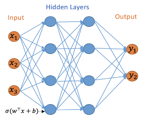
## Neural Network Architecture Diagram: Feedforward Network with Two Hidden Layers ### Overview The image is a technical diagram illustrating the architecture of a feedforward artificial neural network. It visually represents the flow of data from an input layer, through two hidden layers, to an output layer, with all nodes in consecutive layers fully connected. The diagram uses color-coding and mathematical notation to define the network's structure and computational operation. ### Components/Axes The diagram is organized into three distinct vertical sections, labeled at the top: 1. **Input Layer (Left):** Labeled "Input" in orange text. Contains three nodes (circles) colored orange, labeled `x₁`, `x₂`, and `x₃` from top to bottom. 2. **Hidden Layers (Center):** Labeled "Hidden Layers" in blue text. Contains two vertical columns of nodes, each with four blue circles. The columns represent two sequential hidden layers. 3. **Output Layer (Right):** Labeled "Output" in orange text. Contains two nodes (circles) colored orange, labeled `y₁` and `y₂` from top to bottom. **Connections:** Blue arrows connect every node in the Input layer to every node in the first Hidden Layer, every node in the first Hidden Layer to every node in the second Hidden Layer, and every node in the second Hidden Layer to every node in the Output layer. This depicts a "fully connected" or "dense" network topology. **Mathematical Notation:** At the bottom-left corner, near the input layer, the expression `σ(wᵀx + b)` is written in black text. An arrow points from this expression toward the first hidden layer, indicating the fundamental computation performed at each neuron. ### Detailed Analysis * **Layer Dimensions:** * Input Layer: 3 nodes (features: `x₁`, `x₂`, `x₃`). * First Hidden Layer: 4 nodes. * Second Hidden Layer: 4 nodes. * Output Layer: 2 nodes (predictions: `y₁`, `y₂`). * **Topology:** The network is a multilayer perceptron (MLP) with a 3-4-4-2 architecture. The connectivity is exhaustive, with no skipped connections, defining it as a standard feedforward network. * **Activation Function:** The notation `σ(wᵀx + b)` specifies the operation for a single neuron. Here, `x` is the input vector, `w` is the weight vector, `b` is the bias term, `wᵀx` is the dot product, and `σ` (sigma) represents a non-linear activation function (commonly sigmoid, tanh, or ReLU in practice). ### Key Observations 1. **Color Coding:** A consistent color scheme is used: orange for the external interface layers (Input and Output) and blue for the internal processing layers (Hidden Layers). This visually separates the network's boundary from its internal representation. 2. **Symmetry and Density:** The two hidden layers are symmetric in size (4 nodes each). The dense web of blue connection lines emphasizes the high degree of parameterization and the potential for complex feature transformation within the hidden layers. 3. **Notation Placement:** The mathematical formula is placed at the input side, conceptually indicating that this operation is applied as data flows into the first hidden layer and, by extension, to subsequent layers. ### Interpretation This diagram is a canonical representation of a deep neural network's architecture, serving as a blueprint for its information processing pathway. * **Function:** The network is designed to take a 3-dimensional input vector (`x₁, x₂, x₃`), transform it through two successive layers of 4-dimensional non-linear representations, and finally map it to a 2-dimensional output (`y₁, y₂`). This structure is suitable for tasks like binary classification (where `y₁` and `y₂` could represent class probabilities) or regression with two target variables. * **Underlying Principle:** The expression `σ(wᵀx + b)` is the core computational unit. It shows that each blue node computes a weighted sum of its inputs, adds a bias, and then applies a non-linear activation function `σ`. This non-linearity is what allows the network to learn complex, non-linear relationships in data. The repeated application of this operation across layers enables hierarchical feature learning. * **Implied Complexity:** While the diagram is abstract, the dense connectivity implies a large number of trainable parameters (weights and biases). For this specific 3-4-4-2 network, the total number of weights would be (3*4) + (4*4) + (4*2) = 12 + 16 + 8 = 36, plus biases for the 10 non-input nodes, totaling 46 parameters. This highlights the model's capacity to fit intricate patterns. * **Purpose of the Diagram:** It is a pedagogical or design tool meant to communicate the network's structure unambiguously. It abstracts away specific data values and training details to focus purely on the topology and the fundamental mathematical operation that defines a neuron's function.