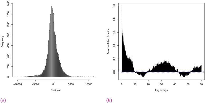
## Histogram and Autocorrelation Plot: Residual Analysis and Temporal Correlation ### Overview The image contains two subplots: **(a)** A histogram of residuals with a bell-shaped distribution. **(b)** An autocorrelation function (ACF) plot showing temporal correlation decay over lag days. --- ### Components/Axes #### Subplot (a): Histogram - **X-axis**: "Residual" (values: -10,000 to 10,000, approximately). - **Y-axis**: "Frequency" (values: 0 to 1,400, approximately). - **Key Feature**: Bell-shaped curve peaking near 0. #### Subplot (b): Autocorrelation Function - **X-axis**: "Lag in days" (values: 0 to 60, approximately). - **Y-axis**: "Autocorrelation function" (values: -1 to 1, approximately). - **Dashed Line**: Horizontal reference at 0.1 (dashed, gray). --- ### Detailed Analysis #### Subplot (a): Histogram - **Distribution**: Symmetric, bell-shaped curve centered at 0. - **Peak Frequency**: Approximately 1,200 (highest bar near 0). - **Tails**: Rapidly decreasing frequency as residuals move away from 0. - **Uncertainty**: Approximate values due to lack of gridlines; peak frequency could range from 1,000–1,400. #### Subplot (b): Autocorrelation Function - **Initial Value**: Sharp peak at lag 0 (~0.8–0.9). - **Decay**: Rapid decline to ~0.2 by lag 10. - **Oscillations**: - First trough: ~-0.2 at lag 10. - Second peak: ~0.3 at lag 20. - Third trough: ~-0.1 at lag 30. - Fourth peak: ~0.15 at lag 40. - Final trough: ~-0.05 at lag 50. - **Significance Threshold**: Dashed line at 0.1; values above this are statistically significant. --- ### Key Observations 1. **Residual Distribution**: Residuals are approximately normally distributed (bell shape), suggesting no systematic bias in the model. 2. **Autocorrelation Decay**: Correlation weakens rapidly after lag 10, but periodic oscillations persist (e.g., peaks at lags 20 and 40). 3. **Significance**: Only the initial peak (lag 0) and lag 20 exceed the 0.1 significance threshold. --- ### Interpretation - **Residual Analysis**: The normal distribution of residuals implies the model’s errors are randomly distributed, supporting its validity. - **Autocorrelation Patterns**: - The decay after lag 10 suggests no strong short-term dependence. - Oscillations (e.g., lag 20, 40) may indicate seasonal or cyclical patterns in the data. - The lack of sustained correlation beyond lag 10 implies the data is likely stationary. - **Practical Implications**: - The model’s residuals are well-behaved, but the autocorrelation oscillations warrant further investigation for hidden temporal dependencies. - The 0.1 threshold helps identify significant lags, but the sparse significant values suggest minimal long-term memory in the data. --- **Note**: All values are approximate due to the absence of gridlines or exact numerical labels. The analysis assumes standard statistical conventions (e.g., ACF significance at 0.1).