## Line Charts: Comparison of Rate Encoding vs. Time Encoding Performance
### Overview
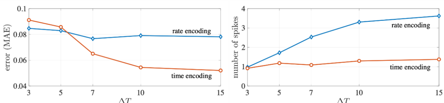
The image contains two side-by-side line charts comparing the performance of two encoding methods—"rate encoding" and "time encoding"—across a variable parameter ΔT. The left chart measures error (Mean Absolute Error, MAE), and the right chart measures the number of spikes. The charts suggest a trade-off between accuracy and computational/spike cost.
### Components/Axes
**Common Elements:**
* **X-Axis (Both Charts):** Labeled "ΔT". The axis markers are at values: 3, 5, 7, 10, and 15.
* **Legend (Both Charts):** Located in the top-right corner of each plot area.
* Blue line with diamond markers: "rate encoding"
* Orange line with circle markers: "time encoding"
**Left Chart:**
* **Title/Y-Axis Label:** "error (MAE)"
* **Y-Axis Scale:** Linear scale ranging from 0.04 to 0.1, with major ticks at 0.04, 0.06, 0.08, and 0.1.
**Right Chart:**
* **Title/Y-Axis Label:** "number of spikes"
* **Y-Axis Scale:** Linear scale ranging from 1 to 4, with major ticks at 1, 2, 3, and 4.
### Detailed Analysis
**Left Chart - Error (MAE) vs. ΔT:**
* **Rate Encoding (Blue, Diamonds):** The trend is relatively flat with a slight initial dip.
* ΔT=3: ~0.085
* ΔT=5: ~0.082
* ΔT=7: ~0.076 (lowest point)
* ΔT=10: ~0.079
* ΔT=15: ~0.078
* **Time Encoding (Orange, Circles):** The trend shows a strong, consistent decrease in error as ΔT increases.
* ΔT=3: ~0.092 (highest point)
* ΔT=5: ~0.085
* ΔT=7: ~0.065
* ΔT=10: ~0.055
* ΔT=15: ~0.052 (lowest point)
**Right Chart - Number of Spikes vs. ΔT:**
* **Rate Encoding (Blue, Diamonds):** The trend shows a strong, consistent increase in the number of spikes as ΔT increases.
* ΔT=3: ~1.5
* ΔT=5: ~1.8
* ΔT=7: ~2.5
* ΔT=10: ~3.3
* ΔT=15: ~3.8 (highest point)
* **Time Encoding (Orange, Circles):** The trend is nearly flat, showing only a very slight increase.
* ΔT=3: ~1.2
* ΔT=5: ~1.5
* ΔT=7: ~1.4
* ΔT=10: ~1.5
* ΔT=15: ~1.5 (plateau)
### Key Observations
1. **Inverse Error Trend:** The two encoding methods show opposite trends in error. Time encoding's error improves (decreases) significantly with larger ΔT, while rate encoding's error remains relatively constant.
2. **Divergent Spike Cost:** The spike cost behavior is also opposite. Rate encoding's spike count grows nearly linearly with ΔT, while time encoding's spike count remains low and stable.
3. **Crossover Point:** For error (left chart), the lines cross between ΔT=5 and ΔT=7. At ΔT=7 and beyond, time encoding has a lower MAE than rate encoding.
4. **Efficiency:** Time encoding appears more efficient for larger ΔT values, achieving lower error without a corresponding increase in spike count.
### Interpretation
This data demonstrates a fundamental performance trade-off between two neural coding schemes. **Rate encoding**, which represents information in the average firing rate, shows stable but mediocre accuracy that comes at a high and growing cost in terms of spike count (energy, bandwidth) as the time window (ΔT) increases.
**Time encoding**, which represents information in the precise timing of spikes, exhibits a different profile. Its accuracy improves dramatically with a longer integration window (larger ΔT), while its spike count remains minimal and constant. This suggests time encoding is a more efficient code for this task, especially when longer processing windows are available. The data implies that for systems where energy efficiency (minimizing spikes) is critical, or where higher accuracy is desired with longer time constants, time encoding is the superior strategy. The stable spike count of time encoding is a particularly notable advantage for scalable neuromorphic hardware.