## Chart: Cumulative Distribution Function of E2E Latency
### Overview
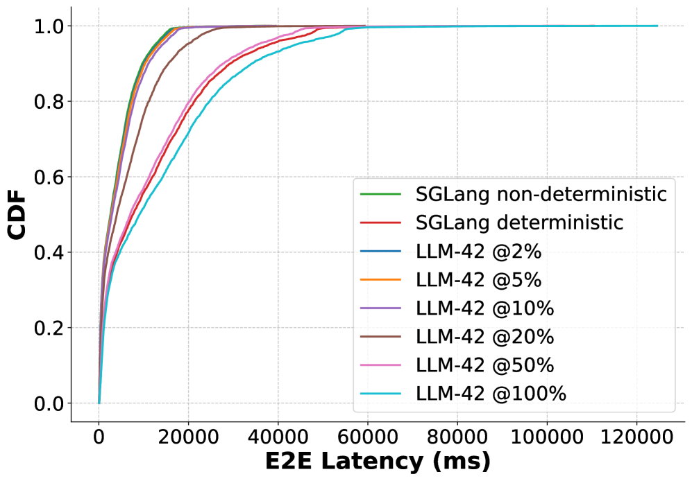
The image presents a cumulative distribution function (CDF) plot illustrating the relationship between E2E Latency (in milliseconds) and the Cumulative Distribution Function (CDF) value, ranging from 0.0 to 1.0. The chart compares the latency distributions of two models, SGLang (deterministic and non-deterministic) and LLM-42, across different sampling percentages (2%, 5%, 10%, 20%, 50%, and 100%).
### Components/Axes
* **X-axis:** E2E Latency (ms), ranging from 0 to 120000 ms.
* **Y-axis:** CDF, ranging from 0.0 to 1.0.
* **Legend:** Located in the top-right corner, identifies the different data series:
* SGLang non-deterministic (Green)
* SGLang deterministic (Red)
* LLM-42 @2% (Blue)
* LLM-42 @5% (Orange)
* LLM-42 @10% (Purple)
* LLM-42 @20% (Brown)
* LLM-42 @50% (Pink)
* LLM-42 @100% (Light Blue)
### Detailed Analysis
The chart displays several CDF curves. Here's a breakdown of each series and approximate data points:
* **SGLang non-deterministic (Green):** This line starts at approximately CDF 0.0 at E2E Latency 0 ms, rapidly increases to CDF 0.5 around 10000 ms, and reaches CDF 0.9 around 30000 ms. It plateaus near CDF 1.0 around 50000 ms.
* **SGLang deterministic (Red):** This line begins at CDF 0.0 at E2E Latency 0 ms, rises to CDF 0.5 around 15000 ms, and reaches CDF 0.9 around 40000 ms. It plateaus near CDF 1.0 around 60000 ms.
* **LLM-42 @2% (Blue):** Starts at CDF 0.0 at E2E Latency 0 ms, reaches CDF 0.5 around 25000 ms, and CDF 0.9 around 60000 ms. It approaches CDF 1.0 around 80000 ms.
* **LLM-42 @5% (Orange):** Begins at CDF 0.0 at E2E Latency 0 ms, reaches CDF 0.5 around 15000 ms, and CDF 0.9 around 50000 ms. It approaches CDF 1.0 around 70000 ms.
* **LLM-42 @10% (Purple):** Starts at CDF 0.0 at E2E Latency 0 ms, reaches CDF 0.5 around 10000 ms, and CDF 0.9 around 40000 ms. It approaches CDF 1.0 around 60000 ms.
* **LLM-42 @20% (Brown):** Begins at CDF 0.0 at E2E Latency 0 ms, reaches CDF 0.5 around 7000 ms, and CDF 0.9 around 30000 ms. It approaches CDF 1.0 around 50000 ms.
* **LLM-42 @50% (Pink):** Starts at CDF 0.0 at E2E Latency 0 ms, reaches CDF 0.5 around 5000 ms, and CDF 0.9 around 25000 ms. It approaches CDF 1.0 around 40000 ms.
* **LLM-42 @100% (Light Blue):** Begins at CDF 0.0 at E2E Latency 0 ms, reaches CDF 0.5 around 3000 ms, and CDF 0.9 around 20000 ms. It approaches CDF 1.0 around 35000 ms.
### Key Observations
* Higher sampling percentages for LLM-42 generally result in lower latency (curves shift to the left).
* SGLang deterministic is consistently slower than SGLang non-deterministic.
* LLM-42 @100% has the lowest latency overall.
* The LLM-42 curves show a clear trend: as the sampling percentage decreases, the latency increases.
* SGLang non-deterministic and LLM-42 @50% have similar CDF curves in the 10000-30000ms range.
### Interpretation
This chart demonstrates the trade-off between latency and sampling percentage in LLM-42. Increasing the sampling percentage reduces latency, but potentially at the cost of output diversity or quality. The comparison between SGLang deterministic and non-deterministic suggests that determinism introduces additional latency. The CDF plot allows for a probabilistic assessment of latency; for example, we can estimate the latency below which 90% of requests will fall for each configuration. The data suggests that LLM-42, particularly with higher sampling percentages, offers significantly lower latency compared to SGLang. The differences in CDF curves highlight the varying distributions of latency for each model and sampling configuration, providing valuable insights for optimizing performance based on specific application requirements.