\n
## Line Chart: MSE vs. Pilot Size for Different Algorithms
### Overview
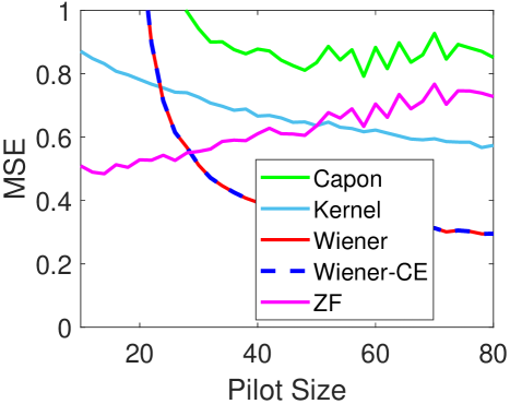
The image presents a line chart illustrating the Mean Squared Error (MSE) as a function of Pilot Size for five different algorithms: Capon, Kernel, Wiener, Wiener-CE, and Zero-Forcing (ZF). The chart aims to compare the performance of these algorithms in terms of MSE as the pilot size varies.
### Components/Axes
* **X-axis:** Pilot Size, ranging from approximately 0 to 80.
* **Y-axis:** MSE (Mean Squared Error), ranging from 0 to 1.
* **Data Series:**
* Capon (Green solid line)
* Kernel (Light Blue solid line)
* Wiener (Red solid line)
* Wiener-CE (Dark Blue dashed line)
* ZF (Magenta solid line)
* **Legend:** Located in the top-right corner of the chart, associating colors with algorithm names.
### Detailed Analysis
Here's a breakdown of each data series and their trends:
* **Capon (Green):** The line starts at approximately 0.9 at a Pilot Size of 0, fluctuates around 0.8-0.9 until approximately Pilot Size 40, then decreases to around 0.75 before increasing again to approximately 0.9 at Pilot Size 80.
* **Kernel (Light Blue):** The line begins at approximately 0.85 at Pilot Size 0, and steadily decreases to approximately 0.6 at Pilot Size 80. The trend is generally downward, but with some fluctuations.
* **Wiener (Red):** The line starts at approximately 0.6 at Pilot Size 0, rapidly decreases to approximately 0.45 at Pilot Size 20, and then plateaus around 0.3-0.4 for Pilot Sizes between 20 and 80.
* **Wiener-CE (Dark Blue):** The line begins at approximately 0.55 at Pilot Size 0, decreases to approximately 0.3 at Pilot Size 20, and then fluctuates between approximately 0.3 and 0.45 for Pilot Sizes between 20 and 80.
* **ZF (Magenta):** The line starts at approximately 0.55 at Pilot Size 0, decreases to approximately 0.4 at Pilot Size 20, and then plateaus around 0.3-0.4 for Pilot Sizes between 20 and 80.
Approximate Data Points (read from the chart):
| Pilot Size | Capon (MSE) | Kernel (MSE) | Wiener (MSE) | Wiener-CE (MSE) | ZF (MSE) |
|---|---|---|---|---|---|
| 0 | 0.9 | 0.85 | 0.6 | 0.55 | 0.55 |
| 20 | 0.85 | 0.75 | 0.45 | 0.3 | 0.4 |
| 40 | 0.8 | 0.7 | 0.4 | 0.4 | 0.35 |
| 60 | 0.8 | 0.65 | 0.35 | 0.4 | 0.35 |
| 80 | 0.9 | 0.6 | 0.3 | 0.4 | 0.3 |
### Key Observations
* The Wiener and Wiener-CE algorithms consistently exhibit the lowest MSE values across most of the Pilot Size range.
* The Capon algorithm has the highest MSE values, particularly at larger Pilot Sizes.
* The Kernel and ZF algorithms show similar performance, with MSE values between those of Capon and Wiener.
* All algorithms show a decreasing MSE as Pilot Size increases, up to a certain point, after which the improvement plateaus or even reverses for Capon.
### Interpretation
The chart demonstrates the trade-off between pilot size and MSE for different signal processing algorithms. Increasing the pilot size generally reduces the MSE, indicating improved performance. However, the rate of improvement diminishes as the pilot size increases, and some algorithms (like Capon) may even experience increased MSE at very large pilot sizes.
The Wiener and Wiener-CE algorithms appear to be the most robust in this scenario, consistently achieving the lowest MSE values. This suggests that these algorithms are less sensitive to the pilot size and provide more reliable performance. The Zero-Forcing algorithm performs similarly to the Kernel algorithm, indicating a comparable level of performance.
The Capon algorithm's higher MSE values suggest that it may be more susceptible to noise or interference, or that it requires a larger pilot size to achieve optimal performance. The fluctuations in the Capon line could indicate instability or sensitivity to specific data characteristics.
The plateauing of the MSE for most algorithms beyond a certain Pilot Size suggests that there is a limit to the performance improvement that can be achieved by simply increasing the pilot size. This could be due to factors such as channel estimation errors or the inherent limitations of the algorithms themselves.