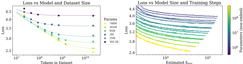
## Chart: Loss vs Model and Dataset Size & Loss vs Model Size and Training Steps ### Overview The image presents two scatter plots side-by-side, both examining the relationship between 'Loss' and other variables. The left plot explores 'Loss' in relation to 'Tokens in Dataset' for different model sizes ('Params'). The right plot explores 'Loss' in relation to 'Estimated Smin' (training steps) for different model sizes ('Params'). The model sizes are color-coded in both plots, allowing for comparison. ### Components/Axes **Left Plot:** * **Title:** Loss vs Model and Dataset Size * **Y-axis:** Loss (linear scale, values ranging from approximately 2.5 to 4.5) * **X-axis:** Tokens in Dataset (logarithmic scale, values ranging from 10^7 to 10^10) * **Legend (Params):** Located on the right side of the left plot. * Yellow: 708M * Light Green: 302M * Green: 85M * Blue: 3M * Dark Blue: 25M * Purple: 393.2K **Right Plot:** * **Title:** Loss vs Model Size and Training Steps * **Y-axis:** Loss (linear scale, values ranging from approximately 2.4 to 4.4) * **X-axis:** Estimated Smin (logarithmic scale, values ranging from 10^4 to 10^5) * **Secondary Y-axis:** Parameters (non-embed) (logarithmic scale, values ranging from 10^6 to 10^8). This axis is represented by a color gradient. * **Color Gradient Legend:** Located on the right side of the right plot. The color gradient maps to the "Parameters (non-embed)" values. Yellow represents lower parameter values, and purple represents higher parameter values. ### Detailed Analysis **Left Plot: Loss vs Model and Dataset Size** * **708M (Yellow):** The loss decreases from approximately 4.3 at 10^7 tokens to approximately 2.7 at 10^10 tokens. * **302M (Light Green):** The loss decreases from approximately 4.1 at 10^7 tokens to approximately 2.9 at 10^10 tokens. * **85M (Green):** The loss decreases from approximately 3.9 at 10^7 tokens to approximately 3.1 at 10^10 tokens. * **3M (Blue):** The loss decreases from approximately 3.7 at 10^7 tokens to approximately 3.3 at 10^10 tokens. * **25M (Dark Blue):** The loss decreases from approximately 4.2 at 10^7 tokens to approximately 3.6 at 10^10 tokens. * **393.2K (Purple):** The loss remains relatively constant, starting at approximately 4.6 at 10^7 tokens and ending at approximately 4.3 at 10^10 tokens. **Trend Verification (Left Plot):** All data series, except for the 393.2K series, show a decreasing trend in loss as the number of tokens in the dataset increases. The 393.2K series remains relatively flat. **Right Plot: Loss vs Model Size and Training Steps** * The data series are color-coded based on the "Parameters (non-embed)" values, ranging from yellow (lower values) to purple (higher values). * All data series show a decreasing trend in loss as the estimated Smin (training steps) increases. * The series with higher parameter values (purple) generally have higher loss values across the range of estimated Smin. * The series with lower parameter values (yellow) generally have lower loss values across the range of estimated Smin. **Trend Verification (Right Plot):** All data series show a decreasing trend in loss as the estimated Smin increases. ### Key Observations * In the left plot, larger models (higher 'Params' values) generally exhibit lower loss for a given number of tokens in the dataset, except for the 393.2K model. * In the right plot, increasing the estimated Smin (training steps) generally leads to a decrease in loss for all model sizes. * The right plot shows a clear correlation between the number of parameters and the loss, with larger models generally having higher loss values. ### Interpretation The plots suggest that increasing both the dataset size (number of tokens) and the number of training steps (estimated Smin) can lead to a reduction in loss. However, the relationship between model size ('Params') and loss is more complex. In the left plot, larger models generally perform better (lower loss) with increasing dataset size. In the right plot, larger models tend to have higher loss values, which could be due to factors such as overfitting or the need for more extensive training. The 393.2K model in the left plot is an outlier, as it does not show a significant decrease in loss with increasing dataset size, suggesting that it may be under-parameterized for the task. The color gradient in the right plot provides a visual representation of how the number of parameters affects the loss, with larger models (purple) generally having higher loss values.

## Charts: Loss vs Model and Dataset Size ### Overview The image presents two charts visualizing the relationship between loss and model/dataset size. The left chart shows Loss vs. Tokens in Dataset, while the right chart shows Loss vs. Estimated S_min (likely a measure of training steps). Both charts use color to represent the number of parameters in the model. ### Components/Axes **Left Chart:** * **Title:** Loss vs Model and Dataset Size * **X-axis:** Tokens in Dataset (log scale, ranging from approximately 10^7 to 10^10) * **Y-axis:** Loss (ranging from approximately 2.5 to 4.5) * **Legend:** Params (color-coded) * 708M (Yellow) * 302M (Green) * 85M (Light Blue) * 3M (Dark Blue) * 25M (Orange) * 393.2K (Purple) **Right Chart:** * **Title:** Loss vs Model Size and Training Steps * **X-axis:** Estimated S_min (log scale, ranging from approximately 10^4 to 10^5) * **Y-axis:** Loss (ranging from approximately 2.4 to 4.4) * **Colorbar:** Parameters (non-embedded) (log scale, ranging from approximately 10^6 to 10^8) - This serves as the legend. ### Detailed Analysis or Content Details **Left Chart:** * **708M (Yellow):** The line starts at approximately Loss = 4.2 with Tokens = 10^7 and decreases rapidly to approximately Loss = 2.6 with Tokens = 10^10. * **302M (Green):** The line starts at approximately Loss = 4.0 with Tokens = 10^7 and decreases to approximately Loss = 3.0 with Tokens = 10^10. * **85M (Light Blue):** The line starts at approximately Loss = 4.1 with Tokens = 10^7 and decreases to approximately Loss = 3.4 with Tokens = 10^10. * **3M (Dark Blue):** The line starts at approximately Loss = 4.3 with Tokens = 10^7 and decreases to approximately Loss = 3.8 with Tokens = 10^10. * **25M (Orange):** The line starts at approximately Loss = 4.1 with Tokens = 10^7 and decreases to approximately Loss = 3.2 with Tokens = 10^10. * **393.2K (Purple):** The line starts at approximately Loss = 4.3 with Tokens = 10^7 and remains relatively flat, ending at approximately Loss = 4.2 with Tokens = 10^10. **Right Chart:** The chart displays a heatmap-like representation of loss as a function of estimated S_min and model parameters. The color intensity corresponds to the number of parameters. * **General Trend:** For all parameter sizes, the loss generally decreases as S_min increases. * **Parameter Impact:** Higher parameter counts (yellow/orange) generally exhibit lower loss values for a given S_min compared to lower parameter counts (blue/purple). * **Specific Observations:** * The highest parameter models (yellow) show the most significant loss reduction with increasing S_min, reaching a loss of approximately 2.4 at S_min = 10^5. * The lowest parameter models (purple) show a less pronounced loss reduction, remaining around a loss of 3.8-4.0 even at S_min = 10^5. ### Key Observations * In the left chart, increasing the dataset size consistently reduces loss across all model sizes. * Larger models (708M, 302M) consistently achieve lower loss values than smaller models (3M, 393.2K) for a given dataset size. * The right chart confirms that increasing training steps (S_min) reduces loss, and this effect is more pronounced for larger models. * The 393.2K model shows minimal improvement with increased dataset size in the left chart, suggesting it may be underparameterized. ### Interpretation The data strongly suggests that both model size and dataset size are critical factors in achieving low loss. Increasing either of these factors leads to improved performance. The right chart reinforces this by showing that increased training (S_min) also contributes to lower loss, particularly for larger models. The consistent trend of decreasing loss with increasing parameters and dataset size indicates a clear scaling relationship. The relatively flat curve for the 393.2K model in the left chart suggests that this model has reached its capacity and cannot benefit further from increased data. This highlights the importance of model capacity in effectively utilizing larger datasets. The colorbar on the right chart provides a continuous representation of parameter size, allowing for a more nuanced understanding of the relationship between model size, training steps, and loss. The logarithmic scales on both axes are appropriate for visualizing the wide range of values involved.

## Chart Type: Dual-Panel Line Charts with Logarithmic Axes ### Overview The image contains two side-by-side line charts analyzing the relationship between model loss, model size, dataset size, and training steps. Both charts use logarithmic scales on their x-axes. The left chart examines loss as a function of dataset size for several fixed model sizes. The right chart examines loss as a function of training steps, with lines colored by model size. The overall theme is the scaling behavior of language models. ### Components/Axes **Left Chart: "Loss vs Model and Dataset Size"** * **Title:** "Loss vs Model and Dataset Size" * **Y-axis:** Label: "Loss". Scale: Linear, from approximately 2.5 to 4.5. Major tick marks at 2.5, 3.0, 3.5, 4.0, 4.5. * **X-axis:** Label: "Tokens in Dataset". Scale: Logarithmic (base 10). Major tick marks and labels at 10⁷, 10⁸, 10⁹, 10¹⁰. * **Legend:** Positioned in the top-right corner. Title: "Params". Contains six entries, each with a colored dot and a label: * Yellow dot: "706M" * Light green dot: "302M" * Green dot: "85M" * Teal dot: "3M" * Dark teal dot: "25M" * Dark purple dot: "393.2K" * **Data Series:** Six dashed lines, each connecting dots of the corresponding legend color. Each line represents a model of a fixed parameter count, showing how its loss decreases as the number of training tokens increases. **Right Chart: "Loss vs Model Size and Training Steps"** * **Title:** "Loss vs Model Size and Training Steps" * **Y-axis:** Label: "Loss". Scale: Linear, from approximately 2.4 to 4.4. Major tick marks at 2.4, 2.8, 3.2, 3.6, 4.0, 4.4. * **X-axis:** Label: "Estimated S_m10". Scale: Logarithmic (base 10). Major tick marks and labels at 10⁴, 10⁵. * **Color Bar (Legend):** Positioned on the far right. Title: "Parameters (non-embed)". Scale: Logarithmic, ranging from 10⁶ to 10⁸. The color gradient runs from dark purple (low parameter count, ~10⁶) through teal and green to yellow (high parameter count, ~10⁸). * **Data Series:** Approximately 20-25 solid lines. Each line represents a training run for a model of a specific size (indicated by its color). The lines show the loss trajectory over training steps (estimated S_m10). ### Detailed Analysis **Left Chart Analysis (Loss vs. Dataset Size):** * **Trend Verification:** All six lines slope downward from left to right, indicating that loss decreases as the number of training tokens increases for all model sizes. The slope is steeper for larger models. * **Data Points (Approximate):** * **706M (Yellow):** Starts at Loss ≈ 4.5 at 10⁷ tokens. Decreases steeply to Loss ≈ 2.4 at 10¹⁰ tokens. * **302M (Light Green):** Starts at Loss ≈ 4.4 at 10⁷ tokens. Decreases to Loss ≈ 2.6 at 10¹⁰ tokens. * **85M (Green):** Starts at Loss ≈ 4.3 at 10⁷ tokens. Decreases to Loss ≈ 2.9 at 10¹⁰ tokens. * **3M (Teal):** Starts at Loss ≈ 4.2 at 10⁷ tokens. Decreases to Loss ≈ 3.1 at 10¹⁰ tokens. * **25M (Dark Teal):** Starts at Loss ≈ 4.1 at 10⁷ tokens. Decreases to Loss ≈ 3.6 at 10¹⁰ tokens. * **393.2K (Dark Purple):** Starts at Loss ≈ 4.6 at 10⁷ tokens. Shows the least improvement, ending at Loss ≈ 4.3 at 10¹⁰ tokens. Its curve is the flattest. **Right Chart Analysis (Loss vs. Training Steps):** * **Trend Verification:** All lines slope downward from left to right, showing that loss decreases with more training steps (estimated S_m10). The lines are roughly parallel in their downward trajectory on the log-linear plot. * **Color-Size Relationship:** Lines colored yellow (high parameter count) are consistently at the bottom of the chart (lowest loss). Lines colored dark purple (low parameter count) are at the top (highest loss). This creates a clear vertical stratification by model size. * **Data Points (Approximate Ranges):** * **Highest Loss (Dark Purple lines, ~10⁶ params):** Start near Loss ≈ 4.4 at 10⁴ steps, decrease to ≈ 4.0 at 10⁵ steps. * **Mid-Range Loss (Teal/Green lines, ~10⁷ params):** Start between Loss ≈ 3.6-4.0 at 10⁴ steps, decrease to ≈ 3.2-3.6 at 10⁵ steps. * **Lowest Loss (Yellow lines, ~10⁸ params):** Start near Loss ≈ 3.0 at 10⁴ steps, decrease to ≈ 2.4 at 10⁵ steps. ### Key Observations 1. **Clear Scaling Laws:** Both charts demonstrate strong, predictable scaling relationships. Loss improves (decreases) with more data (left chart) and more training compute/steps (right chart). 2. **Model Size is Dominant:** In both charts, larger models (more parameters) achieve significantly lower loss at any given point. The vertical separation between lines in the right chart is very pronounced. 3. **Diminishing Returns:** The left chart shows that the rate of loss improvement slows down as dataset size increases (curves flatten slightly on the log scale). This is more dramatic for the smallest model (393.2K). 4. **Consistency Across Views:** The two charts are complementary. The left chart shows the final loss achievable for a model trained on a full dataset of a given size. The right chart shows the path (training dynamics) to get there, confirming that larger models not only reach a lower loss but also maintain a lower loss throughout training. ### Interpretation This data visualizes fundamental scaling principles in machine learning, likely for language models. The charts suggest that **performance (lower loss) is a predictable function of three key resources: model size (parameters), data size (tokens), and training duration (steps).** * **The left chart** implies that to achieve a target loss, one can either train a smaller model on more data or a larger model on less data, but there are limits. The flattening curves, especially for small models, indicate a "data saturation" point where adding more data yields minimal benefit for a fixed model capacity. The 393.2K model appears to saturate very early. * **The right chart** shows the efficiency of training. Larger models (yellow) start at a lower loss and maintain that advantage throughout training. The parallel trajectories suggest that the *rate* of learning (improvement per log-step) might be similar across model sizes, but the starting point and asymptote are determined by model scale. * **The combined message** is one of **predictable scaling**. This type of analysis is crucial for planning resource allocation (compute, data, engineering time) when developing AI systems. It allows practitioners to estimate the expected performance gain from scaling up one dimension (e.g., doubling the dataset) and to identify the most cost-effective scaling strategy. The clear stratification by model size underscores that increasing model capacity is a primary lever for reducing loss, provided sufficient data and training are available.

## Line Charts: Loss vs Model/Dataset Size and Loss vs Model Size/Training Steps ### Overview The image contains two side-by-side line charts analyzing the relationship between model performance (measured as loss) and two key variables: dataset size and training steps. The left chart examines how loss decreases with increasing dataset size for models of varying parameter counts. The right chart explores how loss decreases with increasing training steps (Estimated S_min) for models of different parameter sizes, visualized through a color gradient. ### Components/Axes **Left Chart: Loss vs Model and Dataset Size** - **X-axis**: Tokens in Dataset (log scale, 10⁷ to 10¹⁰) - **Y-axis**: Loss (linear scale, 2.4 to 4.5) - **Legend**: - Yellow: 708M parameters - Green: 302M parameters - Teal: 85M parameters - Blue: 3M parameters - Dark Blue: 25M parameters - Purple: 393.2K parameters - **Line Styles**: Dotted lines for all series; markers (dots) at data points. **Right Chart: Loss vs Model Size and Training Steps** - **X-axis**: Estimated S_min (log scale, 10⁴ to 10⁵) - **Y-axis**: Loss (linear scale, 2.4 to 4.4) - **Color Gradient Legend**: - Yellow (10⁸ parameters) to Purple (10⁶ parameters) - **Line Styles**: Solid lines without markers; grouped by parameter size via color. ### Detailed Analysis **Left Chart Trends**: - All lines show a downward trend: loss decreases as dataset size increases. - Larger models (e.g., 708M, 302M) start with higher loss but achieve lower final loss at larger dataset sizes. - Smaller models (e.g., 393.2K) maintain higher loss across all dataset sizes but show gradual improvement. - Example: At 10¹⁰ tokens, 708M parameters achieve ~2.7 loss, while 393.2K parameters reach ~3.1 loss. **Right Chart Trends**: - All lines slope downward: loss decreases as S_min increases. - Higher-parameter models (yellow) consistently achieve lower loss across all S_min values. - Diminishing returns observed: the steepest loss reduction occurs at lower S_min values (e.g., 10⁴ to 10⁵), with flattening trends at higher S_min. - Example: For 10⁸ parameters (yellow), loss drops from ~3.6 at S_min=10⁴ to ~2.8 at S_min=10⁵. ### Key Observations 1. **Dataset Size Impact**: Larger models benefit more from increased dataset size, achieving lower loss at scale. 2. **Training Steps Impact**: Higher S_min reduces loss, but the effect plateaus for all models, with smaller models showing less improvement. 3. **Parameter-Size Correlation**: Models with more parameters (yellow) outperform smaller models (purple) across both dataset size and training steps. 4. **Diminishing Returns**: Both charts show that gains in performance (loss reduction) slow as variables (tokens/S_min) increase. ### Interpretation The data suggests that model performance (lower loss) is strongly influenced by both dataset size and training steps, with larger models leveraging these resources more effectively. The left chart emphasizes the importance of scaling datasets for complex models, while the right chart highlights the value of extended training, particularly for high-parameter models. However, the diminishing returns in the right chart imply that beyond a certain point, additional training steps yield minimal benefits, especially for smaller models. This underscores a trade-off: investing in larger models or datasets may be more impactful than prolonging training for smaller architectures. The color gradient in the right chart visually reinforces the parameter-size hierarchy, making it easier to compare performance across models.