\n
## Line Graph: MCPS with Processors Configured in a Tree
### Overview
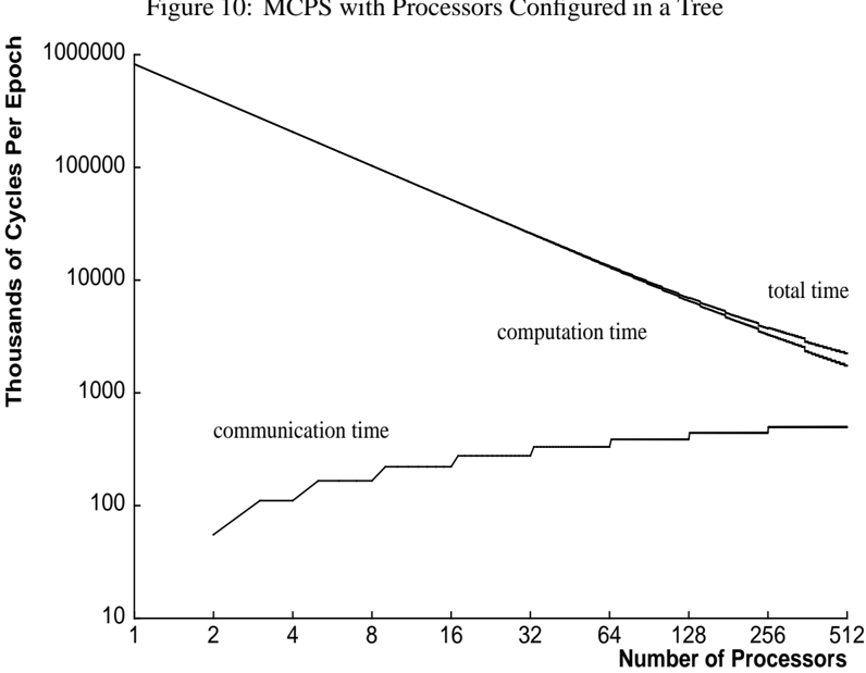
The image is a line graph titled "Figure 10: MCPS with Processors Configured in a Tree." It plots performance metrics (in thousands of cycles per epoch) against the number of processors on a logarithmic scale for both axes. The graph contains three distinct data series representing different time components.
### Components/Axes
* **Title:** "Figure 10: MCPS with Processors Configured in a Tree" (Top center).
* **Y-Axis:** Labeled "Thousands of Cycles Per Epoch". It uses a logarithmic scale with major tick marks at 10, 100, 1000, 10000, 100000, and 1000000.
* **X-Axis:** Labeled "Number of Processors". It uses a logarithmic scale with major tick marks at 1, 2, 4, 8, 16, 32, 64, 128, 256, and 512.
* **Data Series & Legend:** The legend is embedded directly on the graph, with labels placed near their corresponding lines.
1. **"total time"**: The topmost line.
2. **"computation time"**: The middle line, running just below the "total time" line.
3. **"communication time"**: The bottom line, which has a distinct step-like pattern.
### Detailed Analysis
**Trend Verification:**
* **Total Time & Computation Time:** Both lines slope downward from left to right, indicating a decrease in cycles per epoch as the number of processors increases. They follow nearly parallel paths, with "total time" consistently slightly higher than "computation time."
* **Communication Time:** This line slopes upward from left to right in a series of discrete steps, indicating an increase in cycles per epoch as the number of processors increases.
**Data Point Extraction (Approximate Values):**
Values are estimated from the log-log plot. Uncertainty is inherent due to the scale and line thickness.
| Number of Processors | Total Time (Thousands of Cycles) | Computation Time (Thousands of Cycles) | Communication Time (Thousands of Cycles) |
| :--- | :--- | :--- | :--- |
| 1 | ~800,000 | ~780,000 | (Not plotted, starts at 2) |
| 2 | ~400,000 | ~390,000 | ~50 |
| 4 | ~200,000 | ~195,000 | ~100 |
| 8 | ~100,000 | ~97,000 | ~150 |
| 16 | ~50,000 | ~48,000 | ~200 |
| 32 | ~25,000 | ~24,000 | ~250 |
| 64 | ~12,500 | ~12,000 | ~300 |
| 128 | ~6,250 | ~6,000 | ~350 |
| 256 | ~3,125 | ~3,000 | ~400 |
| 512 | ~1,560 | ~1,500 | ~450 |
**Spatial Grounding:** The "communication time" label is positioned in the lower-left quadrant of the plot area, above its corresponding line. The "computation time" label is in the center-right area, just above its line. The "total time" label is in the upper-right area, just above its line.
### Key Observations
1. **Dominant Component:** Computation time is the overwhelming contributor to total time across all processor counts shown.
2. **Diverging Trends:** The gap between the "total time" and "computation time" lines widens slightly as the number of processors increases. This visual gap is filled by the growing "communication time."
3. **Step Function:** Communication time does not increase smoothly; it exhibits clear plateaus and jumps, suggesting that communication overhead increases at specific thresholds in the processor tree configuration (e.g., when moving from 4 to 8, 8 to 16 processors).
4. **Scale of Impact:** While communication time grows, its absolute value (reaching ~450 thousand cycles at 512 processors) remains roughly three orders of magnitude smaller than computation time at that point (~1,500 thousand cycles).
### Interpretation
This graph demonstrates the scalability characteristics of a parallel computing system using a tree processor configuration. The primary insight is that **computation scales nearly perfectly** (the straight downward slope on a log-log plot suggests a power-law relationship, close to ideal linear speedup), as adding more processors drastically reduces the computation time per epoch.
However, the system is not without overhead. The **communication time increases in a stepwise fashion**, revealing the cost of coordinating between processors in the tree. The step pattern likely corresponds to adding new levels or branches to the communication tree, where each jump represents a new tier of processors that must synchronize.
The critical observation is that even at 512 processors, the communication overhead, while growing, is still a small fraction of the total time. This suggests the tree configuration is effective at managing communication costs for the problem being solved (MCPS). The graph implies that for this specific workload and configuration, the system is still in a **computation-dominated regime** within the tested range, and significant further scaling might be possible before communication overhead becomes the primary bottleneck. The widening gap between total and computation time, however, serves as a visual warning of the eventual limit to this scalability.