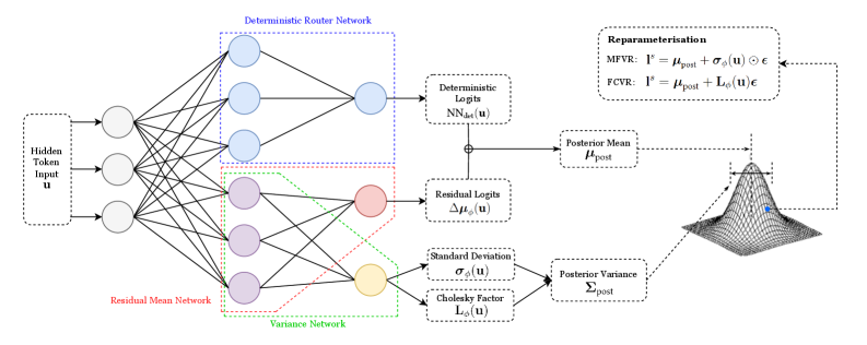
## Diagram: Variational Inference Network ### Overview The image presents a diagram of a variational inference network, illustrating the flow of information from an input token through several network layers to a posterior distribution. The diagram includes components for deterministic routing, residual mean, and variance networks, culminating in a reparameterization step to sample from the posterior. ### Components/Axes * **Input:** Hidden Token Input `u` (located on the left side) * **Deterministic Router Network:** A network block enclosed in a blue dotted rectangle. * **Residual Mean Network:** A network block enclosed in a red dotted rectangle. * **Variance Network:** A network block enclosed in a green dotted rectangle. * **Deterministic Logits:** `NN_det(u)` (top-right, connected to the Deterministic Router Network) * **Residual Logits:** `Δμ_ϕ(u)` (middle-right, connected to the Residual Mean Network) * **Standard Deviation:** `σ_ϕ(u)` (bottom-right, connected to the Variance Network) * **Cholesky Factor:** `L_ϕ(u)` (bottom-right, connected to the Variance Network) * **Posterior Mean:** `μ_post` (right, receives input from Deterministic Logits and Residual Logits) * **Posterior Variance:** `Σ_post` (right, receives input from Standard Deviation and Cholesky Factor) * **Reparameterisation:** * MFVR: `l^s = μ_post + σ_ϕ(u) ⊙ ε` * FCVR: `l^s = μ_post + L_ϕ(u) ε` * **Posterior Distribution:** A 3D Gaussian-like surface plot, with a blue dot indicating the mean. ### Detailed Analysis * **Input Layer:** The Hidden Token Input `u` feeds into three parallel networks. * **Network Layers:** * The Deterministic Router Network outputs to Deterministic Logits `NN_det(u)`. * The Residual Mean Network outputs to Residual Logits `Δμ_ϕ(u)`. * The Variance Network outputs to both Standard Deviation `σ_ϕ(u)` and Cholesky Factor `L_ϕ(u)`. * **Posterior Calculation:** * The Posterior Mean `μ_post` is calculated by combining Deterministic Logits and Residual Logits. * The Posterior Variance `Σ_post` is calculated using Standard Deviation and Cholesky Factor. * **Reparameterisation:** The reparameterization step uses either MFVR or FCVR to sample from the posterior distribution, using the calculated mean and either the standard deviation or Cholesky factor. * **Posterior Distribution Visualization:** The 3D plot visualizes the posterior distribution, with the blue dot indicating the location of the posterior mean. ### Key Observations * The diagram illustrates a variational inference process where the input token is processed through multiple networks to estimate the parameters of a posterior distribution. * The reparameterization trick is used to enable gradient-based learning through the sampling process. * The diagram highlights the modularity of the network, with distinct components for deterministic routing, residual mean, and variance estimation. ### Interpretation The diagram depicts a neural network architecture designed for variational inference. The input `u` is processed through parallel networks to estimate the mean and variance of a posterior distribution. The use of deterministic and residual logits allows for a more flexible and potentially more accurate estimation of the posterior mean. The reparameterization step is crucial for enabling end-to-end training of the network by allowing gradients to flow through the sampling process. The final 3D plot visualizes the learned posterior distribution, providing a qualitative assessment of the network's performance. The MFVR and FCVR equations represent two different ways to reparameterize the distribution, likely corresponding to different assumptions or approximations made during inference.

\n ## Diagram: Neural Network Architecture for Variational Inference ### Overview The image depicts a neural network architecture designed for variational inference. It illustrates the flow of information through a deterministic router network, a residual mean network, and a variance network, culminating in the reparameterization of a distribution. The diagram highlights the key components and their relationships in a probabilistic modeling context. ### Components/Axes The diagram is segmented into three main sections: the input layer, the network layers (Deterministic Router Network, Residual Mean Network, Variance Network), and the reparameterization/output section. * **Input:** "Hidden Token Input u" * **Deterministic Router Network:** Labeled in blue. * **Residual Mean Network:** Labeled in red. * **Variance Network:** Labeled in green. * **Outputs:** * "Deterministic Logits NN_det(u)" * "Residual Logits Δμ_det(u)" * "Standard Deviation σ_det(u)" * "Cholesky Factor L_σ(u)" * **Reparameterisation:** * "MFVR: I^* = μ_post + σ_det(u)ε" * "FCVR: I^* = μ_post + L_σ(u)ε" * **Posterior Distribution:** Visualized as a 3D cone-shaped surface. * "Posterior Mean μ_post" * "Posterior Variance Σ_post" * **ε:** Represents a random variable. ### Detailed Analysis or Content Details The diagram shows a neural network with multiple layers. 1. **Input Layer:** A single input node labeled "Hidden Token Input u". 2. **Deterministic Router Network (Blue):** This network consists of four layers of nodes. The input 'u' is connected to the first layer, which has four nodes. This layer is connected to a second layer with four nodes, then to a third layer with three nodes, and finally to an output layer with two nodes labeled "Deterministic Logits NN_det(u)". 3. **Residual Mean Network (Red):** This network also has four layers of nodes. The input 'u' is connected to the first layer with four nodes, then to a second layer with four nodes, a third layer with three nodes, and finally to an output node labeled "Residual Logits Δμ_det(u)". 4. **Variance Network (Green):** This network has four layers of nodes. The input 'u' is connected to the first layer with four nodes, then to a second layer with four nodes, a third layer with three nodes, and finally to two output nodes labeled "Standard Deviation σ_det(u)" and "Cholesky Factor L_σ(u)". 5. **Reparameterization:** The outputs from the networks are used in the reparameterization formulas for MFVR (Mean-Field Variational Representation) and FCVR (Fully-Connected Variational Representation). Both formulas involve adding a scaled random variable ε to a mean (μ_post). 6. **Posterior Distribution:** The reparameterized output I^* is used to define the posterior distribution, characterized by its mean (μ_post) and variance (Σ_post). The posterior distribution is visualized as a 3D cone-shaped surface. ### Key Observations The diagram emphasizes the use of neural networks to model the posterior distribution in variational inference. The deterministic router network, residual mean network, and variance network work in parallel to estimate the parameters of the posterior distribution. The reparameterization trick is used to enable gradient-based optimization. The visualization of the posterior distribution as a cone suggests a unimodal distribution. ### Interpretation This diagram illustrates a sophisticated approach to variational inference using neural networks. The architecture allows for flexible modeling of complex posterior distributions. The use of separate networks for the mean and variance components enables the model to capture dependencies between these parameters. The reparameterization trick is crucial for enabling gradient-based optimization, which is essential for training the neural networks. The diagram suggests a method for approximating intractable posterior distributions with a more tractable, parameterized form, allowing for efficient inference in Bayesian models. The separation of the deterministic router network suggests a mechanism for controlling the flow of information and potentially improving the accuracy of the approximation. The use of a Cholesky factor for the variance suggests a focus on maintaining positive definiteness, which is important for ensuring the validity of the posterior distribution. The diagram is a high-level overview of a complex system, and further details would be needed to fully understand its implementation and performance.

## Diagram: Probabilistic Neural Network Architecture with Deterministic and Residual Components ### Overview The image is a technical diagram illustrating a neural network architecture designed for probabilistic modeling. It shows the flow of data from a hidden token input through three parallel sub-networks (Deterministic Router, Residual Mean, and Variance Networks) to produce parameters for a posterior distribution, which is then used for reparameterization. The diagram is a flowchart with nodes, connections, and labeled mathematical operations. ### Components/Axes The diagram is organized into a left-to-right flow with distinct, color-coded network components and labeled processing blocks. **1. Input (Far Left):** * **Label:** `Hidden Token Input u` * **Description:** A dashed box representing the input vector `u`. It feeds into three initial nodes (circles). **2. Core Network Components (Center-Left):** Three parallel networks process the input, distinguished by node color and bounding box style. * **Deterministic Router Network:** * **Bounding Box:** Blue dashed rectangle. * **Nodes:** Light blue circles. * **Structure:** A fully connected layer from the 3 input nodes to 3 hidden nodes, then to 1 output node. * **Residual Mean Network:** * **Bounding Box:** Red dashed rectangle. * **Nodes:** Light purple circles. * **Structure:** A fully connected layer from the 3 input nodes to 3 hidden nodes, then to 1 output node (pink circle). * **Variance Network:** * **Bounding Box:** Green dashed rectangle. * **Nodes:** Light purple circles (shared with Residual Mean Network for the first layer), leading to 1 output node (yellow circle). **3. Intermediate Processing Blocks (Center):** * **Deterministic Logits:** A dashed box receiving input from the Deterministic Router Network. Labeled `NN_det(u)`. * **Residual Logits:** A dashed box receiving input from the Residual Mean Network. Labeled `Δμ_post(u)`. * **Standard Deviation:** A dashed box receiving input from the Variance Network. Labeled `σ_post(u)`. * **Cholesky Factor:** A dashed box receiving input from the Variance Network. Labeled `L_σ(u)`. * **Summation Node (⊕):** A circle combining the outputs of `NN_det(u)` and `Δμ_post(u)`. **4. Posterior Distribution Parameters (Center-Right):** * **Posterior Mean:** A dashed box receiving the summed logits. Labeled `μ_post`. * **Posterior Variance:** A dashed box receiving inputs from `σ_post(u)` and `L_σ(u)`. Labeled `Σ_post`. **5. Output & Reparameterisation (Right):** * **Posterior Distribution Visualization:** A 3D wireframe plot of a Gaussian (bell curve) distribution, visually representing the distribution defined by `μ_post` and `Σ_post`. * **Reparameterisation Box:** A large dashed box in the top-right corner containing two equations: * `MPVR: l^s = μ_post + σ_post(u) ⊙ ε` * `FCVR: l^s = μ_post + L_σ(u)ε` ### Detailed Analysis **Flow and Connections:** 1. The `Hidden Token Input u` is fed simultaneously into the three sub-networks. 2. The **Deterministic Router Network** produces a base signal `NN_det(u)`. 3. The **Residual Mean Network** produces a residual adjustment `Δμ_post(u)`. 4. These two are summed to form the final **Posterior Mean `μ_post`**. 5. The **Variance Network** produces two outputs: a standard deviation `σ_post(u)` and a Cholesky factor `L_σ(u)`. 6. These two variance-related outputs are combined to define the **Posterior Variance `Σ_post`**. 7. The parameters `μ_post` and `Σ_post` define a probability distribution (visualized as the 3D bell curve). 8. The **Reparameterisation** box shows how to sample from this distribution (`l^s`) using a noise vector `ε`, using two different methods: MPVR (likely Mean-Parameterised Variance Reparameterisation) and FCVR (likely Full-Covariance Variance Reparameterisation). **Text Transcription (All Labels):** * Hidden Token Input u * Deterministic Router Network * Residual Mean Network * Variance Network * Deterministic Logits * NN_det(u) * Residual Logits * Δμ_post(u) * Standard Deviation * σ_post(u) * Cholesky Factor * L_σ(u) * Posterior Mean * μ_post * Posterior Variance * Σ_post * Reparameterisation * MPVR: l^s = μ_post + σ_post(u) ⊙ ε * FCVR: l^s = μ_post + L_σ(u)ε ### Key Observations 1. **Hybrid Deterministic-Probabilistic Design:** The architecture explicitly separates a deterministic path (Router Network) from probabilistic residual (Mean Network) and variance estimation (Variance Network) paths. 2. **Structured Variance Estimation:** The Variance Network outputs both a standard deviation and a Cholesky factor, suggesting it can model both diagonal and full covariance structures for the posterior distribution. 3. **Residual Learning for the Mean:** The posterior mean is not directly predicted but is formed by adding a residual adjustment (`Δμ_post`) to a deterministic base (`NN_det`). This could stabilize training or allow the model to learn corrections to a strong prior. 4. **Reparameterisation Trick:** The inclusion of the reparameterisation equations confirms this is a variational inference or generative model setup, allowing gradients to flow through stochastic sampling operations. ### Interpretation This diagram depicts a sophisticated **probabilistic layer** for a neural network, likely used in variational autoencoders (VAEs), Bayesian deep learning, or uncertainty estimation tasks. The core innovation appears to be the decoupled estimation of the mean (via a deterministic base + learned residual) and the covariance structure of the approximate posterior distribution. The architecture suggests a design philosophy where: * A **deterministic backbone** (`NN_det`) provides a stable, high-level representation. * A **residual mean network** learns task-specific adjustments to this representation. * A dedicated **variance network** models the uncertainty around this adjusted mean, with the flexibility to capture complex correlations (via the Cholesky factor `L_σ`). The **reparameterisation** step is critical for training, enabling backpropagation through the sampling process. The two formulas (MPVR and FCVR) indicate the model can operate in two modes: one for simpler, possibly diagonal Gaussian posteriors (MPVR), and one for more expressive, full-covariance Gaussian posteriors (FCVR). This architecture would be valuable in scenarios requiring calibrated uncertainty estimates, such as medical diagnosis, autonomous systems, or scientific machine learning.

## Diagram: Variational Autoencoder (VAE) Architecture with Deterministic Router Network ### Overview The diagram illustrates a Variational Autoencoder (VAE) architecture with a deterministic router network. It shows the flow of data from input through multiple neural network components, including residual mean and variance networks, to posterior mean/variance parameters. A Gaussian distribution visualization represents the probabilistic output. ### Components/Axes 1. **Input Layer**: - "Hidden Token Input **u**" 2. **Deterministic Router Network**: - Blue-boxed section with 4 nodes - Outputs to "Deterministic Logits **NN_det(u)**" 3. **Residual Mean Network**: - Red-boxed section with 4 nodes - Outputs to "Residual Logits **Δμ_φ(u)**" 4. **Variance Network**: - Green-boxed section with 4 nodes - Outputs to: - "Standard Deviation **σ_φ(u)**" - "Cholesky Factor **L_φ(u)**" 5. **Posterior Parameters**: - "Posterior Mean **μ_post**" - "Posterior Variance **Σ_post**" 6. **Reparameterization**: - Equations for: - **MFVR**: **l**^s = **μ_post** + **σ_φ(u)** ⊙ **ε** - **FCVR**: **l**^s = **μ_post** + **L_φ(u)** **ε** 7. **Gaussian Distribution**: - Visualized with **μ_post** (mean) and **Σ_post** (variance) ### Spatial Grounding - **Top-left**: Hidden Token Input **u** feeds into all networks - **Center-left**: Deterministic Router Network (blue) - **Center**: Residual Mean Network (red) and Variance Network (green) - **Right**: Posterior parameters and reparameterization equations - **Bottom-right**: Gaussian curve visualization ### Detailed Analysis 1. **Data Flow**: - Input **u** → Deterministic Router Network → Deterministic Logits **NN_det(u)** - Input **u** → Residual Mean Network → Residual Logits **Δμ_φ(u)** - Input **u** → Variance Network → Standard Deviation **σ_φ(u)** and Cholesky Factor **L_φ(u)** - Residual Logits + Variance components → Posterior Mean **μ_post** and Variance **Σ_post** - Posterior parameters used in reparameterization equations 2. **Equations**: - **MFVR** (Mean-Field Variational Reparameterization): **l**^s = **μ_post** + **σ_φ(u)** ⊙ **ε** - **FCVR** (Fully Connected Variational Reparameterization): **l**^s = **μ_post** + **L_φ(u)** **ε** 3. **Gaussian Visualization**: - Blue dot represents sampling point - Curve shape determined by **μ_post** (center) and **Σ_post** (spread) ### Key Observations 1. The deterministic router network acts as a gating mechanism for input distribution 2. Residual and variance networks enable separate modeling of mean and uncertainty 3. Cholesky Factor **L_φ(u)** enables efficient variance parameterization 4. Reparameterization bridges probabilistic and deterministic components 5. Gaussian curve confirms the model's probabilistic output distribution ### Interpretation This architecture demonstrates a hybrid approach combining deterministic routing with probabilistic modeling. The deterministic router network likely enables structured decomposition of input representations, while the residual/variance networks capture uncertainty. The reparameterization equations show how the model balances exploration (via sampling **ε**) with exploitation (via posterior parameters). The Gaussian visualization emphasizes the VAE's core principle of learning data distributions rather than point estimates. The architecture suggests applications in tasks requiring both structured representation learning and uncertainty quantification, such as generative modeling of structured data with inherent variability.