## Diagram: Variational Inference Network
### Overview
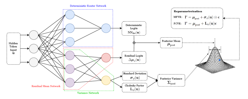
The image presents a diagram of a variational inference network, illustrating the flow of information from an input token through several network layers to a posterior distribution. The diagram includes components for deterministic routing, residual mean, and variance networks, culminating in a reparameterization step to sample from the posterior.
### Components/Axes
* **Input:** Hidden Token Input `u` (located on the left side)
* **Deterministic Router Network:** A network block enclosed in a blue dotted rectangle.
* **Residual Mean Network:** A network block enclosed in a red dotted rectangle.
* **Variance Network:** A network block enclosed in a green dotted rectangle.
* **Deterministic Logits:** `NN_det(u)` (top-right, connected to the Deterministic Router Network)
* **Residual Logits:** `Δμ_ϕ(u)` (middle-right, connected to the Residual Mean Network)
* **Standard Deviation:** `σ_ϕ(u)` (bottom-right, connected to the Variance Network)
* **Cholesky Factor:** `L_ϕ(u)` (bottom-right, connected to the Variance Network)
* **Posterior Mean:** `μ_post` (right, receives input from Deterministic Logits and Residual Logits)
* **Posterior Variance:** `Σ_post` (right, receives input from Standard Deviation and Cholesky Factor)
* **Reparameterisation:**
* MFVR: `l^s = μ_post + σ_ϕ(u) ⊙ ε`
* FCVR: `l^s = μ_post + L_ϕ(u) ε`
* **Posterior Distribution:** A 3D Gaussian-like surface plot, with a blue dot indicating the mean.
### Detailed Analysis
* **Input Layer:** The Hidden Token Input `u` feeds into three parallel networks.
* **Network Layers:**
* The Deterministic Router Network outputs to Deterministic Logits `NN_det(u)`.
* The Residual Mean Network outputs to Residual Logits `Δμ_ϕ(u)`.
* The Variance Network outputs to both Standard Deviation `σ_ϕ(u)` and Cholesky Factor `L_ϕ(u)`.
* **Posterior Calculation:**
* The Posterior Mean `μ_post` is calculated by combining Deterministic Logits and Residual Logits.
* The Posterior Variance `Σ_post` is calculated using Standard Deviation and Cholesky Factor.
* **Reparameterisation:** The reparameterization step uses either MFVR or FCVR to sample from the posterior distribution, using the calculated mean and either the standard deviation or Cholesky factor.
* **Posterior Distribution Visualization:** The 3D plot visualizes the posterior distribution, with the blue dot indicating the location of the posterior mean.
### Key Observations
* The diagram illustrates a variational inference process where the input token is processed through multiple networks to estimate the parameters of a posterior distribution.
* The reparameterization trick is used to enable gradient-based learning through the sampling process.
* The diagram highlights the modularity of the network, with distinct components for deterministic routing, residual mean, and variance estimation.
### Interpretation
The diagram depicts a neural network architecture designed for variational inference. The input `u` is processed through parallel networks to estimate the mean and variance of a posterior distribution. The use of deterministic and residual logits allows for a more flexible and potentially more accurate estimation of the posterior mean. The reparameterization step is crucial for enabling end-to-end training of the network by allowing gradients to flow through the sampling process. The final 3D plot visualizes the learned posterior distribution, providing a qualitative assessment of the network's performance. The MFVR and FCVR equations represent two different ways to reparameterize the distribution, likely corresponding to different assumptions or approximations made during inference.