## Distribution Comparison Chart: e4-mid Distribution Comparison
### Overview
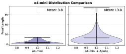
The image displays a side-by-side comparison of two statistical distributions, likely representing pixel intensity or value distributions from two different datasets or conditions labeled "e4" and "mid". The chart uses filled area plots (similar to violin plots or kernel density estimates) to visualize the shape and spread of each distribution. The overall aesthetic is a clean, scientific plot with a white background and black axes.
### Components/Axes
* **Main Title:** "e4-mid Distribution Comparison" (centered at the top).
* **Left Plot:**
* **Annotation:** "Mean: 3.8" (positioned at the top-center of the left plot area).
* **Y-axis Label:** "Pixel Count" (rotated vertically on the left side).
* **Y-axis Scale:** Linear scale from 0 to 60, with major tick marks at 0, 20, 40, and 60.
* **X-axis:** No explicit label. The scale runs from 0.0 to 1.2, with major tick marks at 0.0, 0.2, 0.4, 0.6, 0.8, 1.0, and 1.2.
* **Data Representation:** A filled area plot in a light, desaturated blue/purple color. The distribution is widest (highest pixel count) at the lower end of the x-axis and tapers off as x increases.
* **Right Plot:**
* **Annotation:** "Mean: 13.0" (positioned at the top-center of the right plot area).
* **Y-axis Label:** "Pixel Count" (shared with the left plot, implied by alignment).
* **Y-axis Scale:** Identical to the left plot (0 to 60).
* **X-axis:** No explicit label. The scale runs from 0.0 to 1.5, with major tick marks at 0.0, 0.5, 1.0, and 1.5.
* **Data Representation:** A filled area plot in a darker, more saturated purple color. The distribution has a pronounced, sharp peak in the middle of its range and is narrower overall compared to the left plot.
### Detailed Analysis
* **Left Distribution (e4?):**
* **Trend:** The distribution is right-skewed. It has its maximum density (peak pixel count) at a low x-value, approximately between 0.1 and 0.3. The pixel count decreases steadily as the x-value increases towards 1.2.
* **Key Data Points (Approximate):**
* Peak Pixel Count: ~15-20 (at x ≈ 0.2).
* Pixel Count at x=0.0: ~5.
* Pixel Count at x=0.6: ~2.
* Pixel Count at x=1.0: Approaching 0.
* **Central Tendency:** The mean is explicitly stated as 3.8.
* **Right Distribution (mid?):**
* **Trend:** The distribution is roughly symmetric and leptokurtic (peaked). It rises sharply to a high peak and then falls symmetrically.
* **Key Data Points (Approximate):**
* Peak Pixel Count: ~55 (at x ≈ 0.7).
* Pixel Count at x=0.0: ~0.
* Pixel Count at x=0.5: ~20.
* Pixel Count at x=1.0: ~20.
* Pixel Count at x=1.5: Approaching 0.
* **Central Tendency:** The mean is explicitly stated as 13.0.
### Key Observations
1. **Contrasting Shapes:** The two distributions are fundamentally different. The left plot shows a broad, decaying distribution concentrated at low values, while the right plot shows a narrow, peaked distribution centered at a higher value.
2. **Mean Discrepancy:** The mean of the right distribution (13.0) is significantly higher than that of the left (3.8), confirming the visual shift of mass to the right.
3. **Peak Density:** The peak pixel count in the right distribution (~55) is nearly three times higher than the peak in the left distribution (~15-20), indicating a much higher concentration of data points around its central value.
4. **Range:** The left distribution's meaningful data spans from x=0.0 to ~1.0. The right distribution's meaningful data spans from x=0.2 to ~1.2, with its core between 0.5 and 1.0.
### Interpretation
This chart effectively demonstrates a stark contrast between two data populations. The "e4" (left) distribution suggests a dataset where most values are low, with a long tail of less frequent higher values—characteristic of noise, background, or a process with a lower baseline. The "mid" (right) distribution suggests a dataset with a strong, consistent signal centered around a specific value (x≈0.7), with little deviation—characteristic of a focused measurement, a detected feature, or a processed signal.
The comparison likely aims to show the effect of a process (e.g., image processing, filtering, or segmentation). The "mid" distribution could represent the result of isolating a specific feature (like a cell or object in an image) from the broader, noisier background represented by the "e4" distribution. The higher mean and peaked shape indicate successful concentration and enhancement of the signal of interest. The clear separation in both mean and distribution shape suggests the two conditions or datasets are distinctly different and the process being visualized has a dramatic effect on the data's statistical properties.