## Scatter Plot and Decision Tree: Census Income Data
### Overview
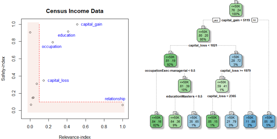
The image presents two distinct visualizations related to census income data. On the left, a scatter plot displays the "Safety-index" against the "Relevance-index" for various factors like capital gain, education, occupation, capital loss, and relationship. A shaded region is present in the bottom-left corner. On the right, a decision tree illustrates how different features (capital gain, capital loss, occupation, education) are used to predict income levels (<=50K or >50K).
### Components/Axes
**Left: Scatter Plot**
* **Title:** Census Income Data
* **X-axis:** Relevance-index, ranging from 0.0 to 1.0 in increments of 0.2.
* **Y-axis:** Safety-index, ranging from 0.0 to 1.0 in increments of 0.2.
* **Data Points:**
* capital\_gain: Located at approximately (0.5, 0.9).
* education: Located at approximately (0.4, 0.8).
* occupation: Located at approximately (0.3, 0.7).
* capital\_loss: Located at approximately (0.2, 0.35).
* relationship: Located at approximately (0.9, 0.15).
* **Shaded Region:** A light red shaded rectangular region exists in the bottom-left corner, bounded by x=0 to x=0.2 and y=0 to y=0.1.
**Right: Decision Tree**
* The tree predicts income levels (<=50K or >50K) based on various features.
* Each node contains information about the predicted income level, the percentage split, and the percentage of data points reaching that node.
* Decision nodes split based on conditions like "capital\_gain < 5119", "capital\_loss < 1821", "occupationExec-managerial < 0.5", "educationMasters < 0.5", and "capital\_loss < 2365".
### Detailed Analysis
**Left: Scatter Plot**
* The scatter plot shows the relative "Safety-index" and "Relevance-index" of different factors.
* "capital\_gain" has the highest Safety-index and a relatively high Relevance-index.
* "relationship" has the highest Relevance-index but a low Safety-index.
* "capital\_loss" has low values for both indices.
**Right: Decision Tree**
* **Root Node (Node 1):** If capital\_gain is less than 5119, 76% of the samples are <=50K and 24% are >50K. This node accounts for 100% of the data.
* **Node 2:** If capital\_gain >= 5119, and capital\_loss is less than 1821, 80% of the samples are <=50K and 20% are >50K. This node accounts for 95% of the data.
* **Node 5:** If capital\_gain >= 5119, and capital\_loss is greater than or equal to 1979, 28% of the samples are <=50K and 72% are >50K. This node accounts for 3% of the data.
* **Node 4:** If capital\_gain < 5119, 81% of the samples are <=50K and 19% are >50K. This node accounts for 92% of the data.
* **Node 8:** If capital\_gain < 5119, capital\_loss < 1821, and occupationExec-managerial is less than 0.5, 84% of the samples are <=50K and 16% are >50K. This node accounts for 82% of the data.
* **Node 16:** If capital\_gain < 5119, capital\_loss < 1821, and occupationExec-managerial is greater than or equal to 0.5, 64% of the samples are <=50K and 36% are >50K. This node accounts for 9% of the data.
* **Node 9:** If capital\_gain < 5119, capital\_loss >= 1979, and educationMasters is less than 0.5, 35% of the samples are <=50K and 65% are >50K. This node accounts for 1% of the data.
* **Node 20:** If capital\_gain < 5119, capital\_loss >= 1979, and educationMasters is greater than or equal to 0.5, 85% of the samples are <=50K and 15% are >50K. This node accounts for 1% of the data.
* **Node 21:** If capital\_gain >= 5119, capital\_loss >= 1979, and capital\_loss < 2365, 21% of the samples are <=50K and 79% are >50K. This node accounts for 0% of the data.
* **Node 11:** If capital\_gain >= 5119, capital\_loss >= 1979, and capital\_loss >= 2365, 11% of the samples are <=50K and 89% are >50K. This node accounts for 2% of the data.
* **Node 3:** If capital\_gain >= 5119, capital\_loss >= 1979, 5% of the samples are <=50K and 95% are >50K. This node accounts for 5% of the data.
### Key Observations
* The scatter plot provides a high-level overview of the importance and safety of different factors related to income.
* The decision tree shows how these factors can be used to predict income levels.
* Capital gain appears to be the most important factor in determining income level, as it is the first split in the decision tree.
* Capital loss, occupation, and education also play a role in predicting income level.
### Interpretation
The data suggests that capital gain is a strong indicator of income level. Individuals with higher capital gains are more likely to have an income greater than $50,000. Other factors, such as capital loss, occupation, and education, also contribute to the prediction of income level, but to a lesser extent. The decision tree provides a model for predicting income level based on these factors. The scatter plot provides a visual representation of the relative importance and safety of these factors. The shaded region in the bottom-left of the scatter plot likely indicates a region of low relevance and low safety, suggesting that factors falling within this region are not significant predictors of income.