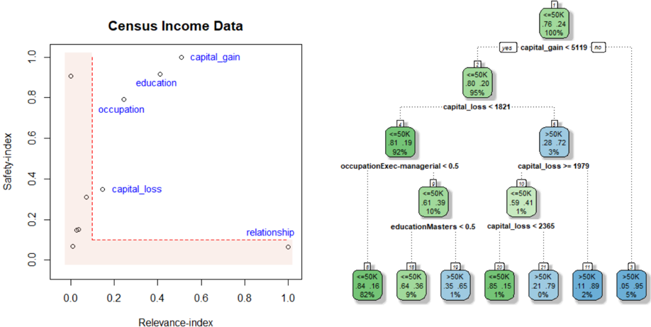
\n ## Scatter Plot & Mosaic Plots: Census Income Data ### Overview The image presents a scatter plot alongside a series of mosaic plots (also known as treemaps or Marimekko charts). The scatter plot visualizes the relationship between "Relevance-index" and "Safety-index" for different factors related to census income data: "capital_gain", "education", "occupation", "capital_loss", and "relationship". The mosaic plots break down the distribution of income levels (<=50K and >50K) based on combinations of these factors. ### Components/Axes * **Scatter Plot:** * X-axis: Relevance-index (Scale: 0.0 to 1.0) * Y-axis: Safety-index (Scale: 0.0 to 1.0) * Data Points: Labeled as "capital_gain", "education", "occupation", "capital_loss", and "relationship". * **Mosaic Plots:** Each plot represents a specific combination of factors and income level. * The width of each rectangle represents the proportion of individuals in that category. * The rectangles are divided into two sections, representing income levels: <=50K and >50K. * Each section displays the percentage of individuals within that income level for the given category. * **Legend:** Located in the top-right corner, indicating income levels: "yes" (<=50K) and "no" (>50K). The colors are white and dark gray respectively. ### Detailed Analysis or Content Details **Scatter Plot:** * **capital_gain:** Located approximately at (0.3, 0.3). * **education:** Located approximately at (0.2, 0.7). * **occupation:** Located approximately at (0.3, 0.5). * **capital_loss:** Located approximately at (0.1, 0.2). * **relationship:** Located approximately at (0.9, 0.1). **Mosaic Plots (from top to bottom, left to right):** 1. **capital_gain < 5119:** * <=50K: 78%, 24 individuals * >50K: 100% 2. **capital_loss < 1821:** * <=50K: 81%, 19 individuals * >50K: 80%, 20 individuals * Total: 95% 3. **occupationExec-managerial < 0.5:** * <=50K: 81%, 19 individuals * >50K: 28%, 72 individuals * Total: 92% 4. **capital_loss >= 1979:** * <=50K: 61%, 39 individuals * >50K: 59%, 41 individuals * Total: 10% 5. **educationMasters < 0.5:** * <=50K: 84%, 16 individuals * >50K: 64%, 36 individuals * Total: 82% 6. **capital_gain >= 2365:** * <=50K: 85%, 15 individuals * >50K: 21%, 79 individuals * Total: 1% 7. **<=50K:** * <=50K: 35%, 65 individuals * >50K: 11%, 89 individuals * Total: 2% 8. **>50K:** * <=50K: 0%, 0 individuals * >50K: 95%, 5 individuals * Total: 5% ### Key Observations * The scatter plot suggests a weak or non-linear relationship between the Relevance-index and Safety-index for the factors considered. "relationship" has a high Relevance-index and low Safety-index. * The mosaic plots reveal varying distributions of income levels across different factor combinations. * The "capital_gain < 5119" plot shows a strong association with >50K income. * The "capital_loss >= 1979" plot shows a relatively even distribution between <=50K and >50K income. * The "educationMasters < 0.5" plot shows a higher proportion of individuals with <=50K income. * The last two mosaic plots show a very skewed distribution of income levels. ### Interpretation The image presents an exploratory data analysis of census income data, attempting to identify factors that correlate with income level. The scatter plot provides a high-level overview of the relationships between different factors and their relevance/safety indices. The mosaic plots offer a more granular view, revealing how specific combinations of factors influence income distribution. The strong association between "capital_gain < 5119" and >50K income suggests that individuals with lower capital gains are more likely to earn higher incomes. Conversely, the relatively even distribution in the "capital_loss >= 1979" plot indicates that capital loss may not be a strong predictor of income level. The "educationMasters < 0.5" plot suggests that individuals with a Master's degree but a low score on the education index are more likely to earn <=50K. The skewed distributions in the final two mosaic plots (<=50K and >50K) suggest that these income levels are heavily influenced by specific factor combinations. The fact that the >50K plot has a high proportion of individuals (95%) indicates a strong positive correlation between the factors considered and high income. The overall analysis suggests that income level is a complex phenomenon influenced by multiple factors, and that certain combinations of factors are more strongly associated with income than others. Further investigation would be needed to determine the causal relationships between these factors and income level.