\n
## Scatter Plot & Decision Tree: Census Income Data Analysis
### Overview
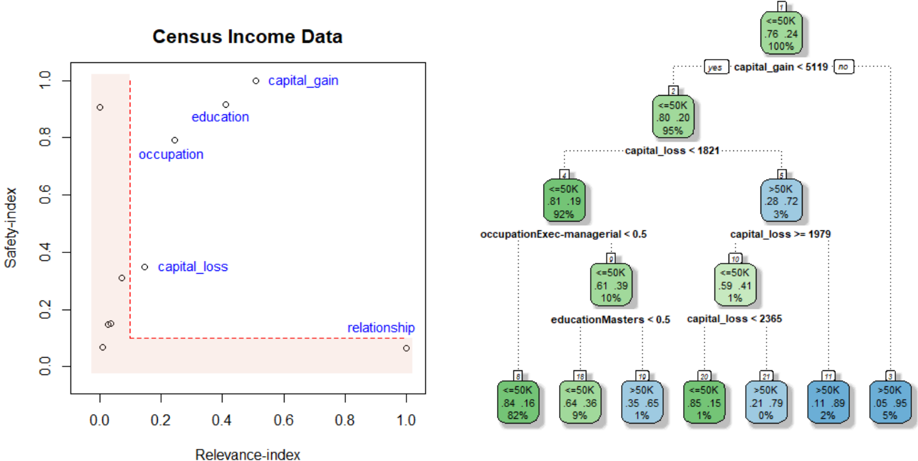
The image presents a two-part technical analysis of the "Census Income Data" dataset. On the left is a scatter plot comparing features based on "Relevance-index" and "Safety-index." On the right is a decision tree classifier predicting income (<=50K vs. >50K) based on those features. The visualization aims to correlate feature importance (relevance) with a fairness or bias metric (safety) and show how those features are used in a predictive model.
### Components/Axes
**Left: Scatter Plot**
* **Title:** "Census Income Data"
* **X-axis:** "Relevance-index" (Scale: 0.0 to 1.0, with ticks at 0.0, 0.2, 0.4, 0.6, 0.8, 1.0)
* **Y-axis:** "Safety-index" (Scale: 0.0 to 1.0, with ticks at 0.0, 0.2, 0.4, 0.6, 0.8, 1.0)
* **Data Points:** Five labeled points representing dataset features:
* `capital_gain`
* `education`
* `occupation`
* `capital_loss`
* `relationship`
* **Other Elements:** A shaded, light-red region in the bottom-left quadrant, bounded by a dashed red line. This likely indicates a zone of low relevance and low safety.
**Right: Decision Tree Diagram**
* **Structure:** A hierarchical tree with nodes and branches. Branches are labeled "yes" or "no" for the decision condition.
* **Node Content:** Each node displays:
* Predicted class: `<=50K` (green background) or `>50K` (blue background).
* Class distribution (two decimal percentages).
* Percentage of total samples reaching that node.
* **Decision Rules (from top to bottom):**
1. `capital_gain <= 5119`
2. `capital_loss < 1821`
3. `occupationExec-managerial < 0.5`
4. `educationMasters < 0.5`
5. `capital_loss >= 1979`
6. `capital_loss < 2365`
### Detailed Analysis
**Scatter Plot Analysis:**
* **Trend:** There is a clear negative correlation. Features with high Relevance-index have low Safety-index, and vice-versa.
* **Data Points (Approximate Coordinates):**
* `capital_gain`: (Relevance: ~0.95, Safety: ~0.95) - *Most relevant, least safe.*
* `education`: (Relevance: ~0.45, Safety: ~0.85)
* `occupation`: (Relevance: ~0.35, Safety: ~0.75)
* `capital_loss`: (Relevance: ~0.15, Safety: ~0.35)
* `relationship`: (Relevance: ~1.0, Safety: ~0.05) - *Highest relevance, lowest safety.*
* **Spatial Grounding:** The labeled points are scattered from the top-left (`capital_gain`) to the bottom-right (`relationship`). The shaded region occupies the area where both indices are below ~0.1.
**Decision Tree Content Details:**
* **Root Node (Top Center):** Predicts `<=50K` (76% / 24% distribution) for 100% of samples. Splits on `capital_gain <= 5119`.
* **Level 1 Nodes:**
* **Left (Yes):** Predicts `<=50K` (80% / 20%) for 95% of samples. Splits on `capital_loss < 1821`.
* **Right (No):** Predicts `>50K` (28% / 72%) for 5% of samples. This is a leaf node.
* **Level 2 Nodes (from Left Node):**
* **Left (Yes):** Predicts `<=50K` (81% / 19%) for 92% of samples. Splits on `occupationExec-managerial < 0.5`.
* **Right (No):** Predicts `>50K` (59% / 41%) for 1% of samples. Splits on `capital_loss >= 1979`.
* **Level 3 Nodes & Leaves:**
* From `occupationExec-managerial < 0.5`:
* **Left (Yes):** Leaf. Predicts `<=50K` (84% / 16%) for 82% of samples.
* **Right (No):** Splits on `educationMasters < 0.5`.
* **Left (Yes):** Leaf. Predicts `<=50K` (64% / 36%) for 9% of samples.
* **Right (No):** Leaf. Predicts `>50K` (35% / 65%) for 1% of samples.
* From `capital_loss >= 1979`:
* **Left (Yes):** Leaf. Predicts `<=50K` (85% / 15%) for 1% of samples.
* **Right (No):** Splits on `capital_loss < 2365`.
* **Left (Yes):** Leaf. Predicts `>50K` (21% / 79%) for 0% of samples (very few).
* **Right (No):** Leaf. Predicts `>50K` (11% / 89%) for 2% of samples.
* **Final Leaf (far right):** Predicts `>50K` (05% / 95%) for 5% of samples. *(Note: This appears to be a separate leaf from the main tree path, possibly connected to the initial `capital_gain > 5119` branch).*
### Key Observations
1. **Feature Trade-off:** The scatter plot reveals a fundamental tension: the features most predictive of income (`capital_gain`, `relationship`) are also the ones with the lowest "Safety-index," suggesting they may be proxies for sensitive attributes or introduce bias.
2. **Tree Logic:** The decision tree heavily prioritizes `capital_gain` as the primary splitter. A high capital gain (>5119) immediately classifies an individual into the >50K income bracket with high confidence (72%).
3. **Path to >50K:** The primary path to a >50K prediction involves having a low capital gain but a high capital loss (>=1979) and not being in an executive-managerial occupation.
4. **Class Imbalance:** The root node shows the dataset is imbalanced, with 76% of samples earning <=50K.
### Interpretation
This visualization performs a dual analysis: **exploratory** (scatter plot) and **explanatory** (decision tree).
* **What the data suggests:** The scatter plot suggests that using the most "relevant" features for accuracy (`capital_gain`, `relationship`) may come at the cost of model "safety" (fairness, lack of bias). This is a classic accuracy-fairness trade-off in machine learning.
* **How elements relate:** The decision tree operationalizes the features from the scatter plot. It confirms `capital_gain`'s high relevance by placing it at the root. The tree's structure shows how combinations of features (like `capital_loss` and `occupation`) are used to refine predictions, but the most decisive factor is a single, high-value financial indicator.
* **Notable Anomalies:** The `relationship` feature has the highest relevance but lowest safety. In the tree, it does not appear as a direct node, implying its predictive power might be captured indirectly through other splits or that it was excluded from this specific tree model due to its low safety score. The shaded "low-low" region in the scatter plot contains no labeled features, suggesting the model avoids using features that are both irrelevant and unsafe.
**Language:** All text in the image is in English.