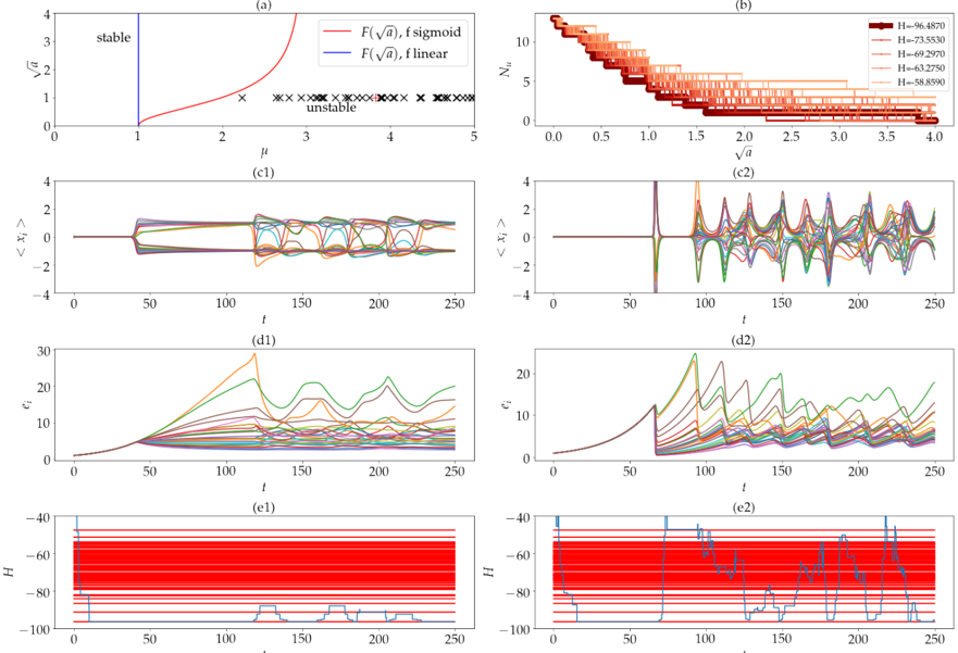
## Chart/Diagram Type: Multi-Panel Figure ### Overview The image is a multi-panel figure consisting of six subplots, arranged in a 3x2 grid. The subplots display various relationships between parameters, including stability analysis, population dynamics, and energy levels. The figure explores the behavior of a system under different conditions, likely related to a physical or biological model. ### Components/Axes **Panel (a): Stability Diagram** * **X-axis:** μ (mu), ranging from 0 to 5. * **Y-axis:** √a (square root of a), ranging from 0 to 4. * **Curves:** * Red line: F(√a), f sigmoid * Blue line: F(√a), f linear * **Regions:** * "stable" region to the left of the blue line (μ ≈ 1). * "unstable" region indicated by black 'x' marks to the right of the red line. **Panel (b): Population Dynamics** * **X-axis:** √a (square root of a), ranging from 0 to 4. * **Y-axis:** N_u, ranging from 0 to 12. * **Curves:** Multiple lines representing different values of H (energy), ranging from -96.4870 to -58.8590. The lines are colored in shades of brown, with darker shades representing lower H values. * H = -96.4870 (darkest brown) * H = -73.5530 * H = -69.2970 * H = -63.2750 * H = -58.8590 (lightest brown) **Panel (c1) and (c2): Time Series of <x_i>** * **X-axis:** t (time), ranging from 0 to 250. * **Y-axis:** <x_i>, ranging from -4 to 4. * **Curves:** Multiple lines, each representing a different instance or component of the system. **Panel (d1) and (d2): Time Series of e_i** * **X-axis:** t (time), ranging from 0 to 250. * **Y-axis:** e_i, ranging from 0 to 30. * **Curves:** Multiple lines, each representing a different instance or component of the system. **Panel (e1) and (e2): Time Series of H** * **X-axis:** t (time), ranging from 0 to 250. * **Y-axis:** H (energy), ranging from -100 to -40. * **Curves:** * Multiple red lines clustered around -60. * A single blue line showing fluctuations in energy. ### Detailed Analysis or ### Content Details **Panel (a): Stability Diagram** * The blue line (F(√a), f linear) is a vertical line at μ ≈ 1, indicating a sharp transition to instability. * The red line (F(√a), f sigmoid) curves upward, showing that the system becomes unstable at lower √a values as μ increases. * The region to the left of the blue line is labeled "stable," while the region to the right of the red line is marked with "x" symbols and labeled "unstable." **Panel (b): Population Dynamics** * The number of populations, N_u, decreases as √a increases. * The different H values (energy levels) influence the rate of decrease in N_u. Lower H values (darker brown lines) show a steeper decrease in N_u as √a increases. * The lines show a step-wise decrease, suggesting discrete population levels. **Panel (c1) and (c2): Time Series of <x_i>** * In panel (c1), the lines start at approximately 0 and then diverge around t=50, oscillating before settling to a value between -2 and 2. * In panel (c2), the lines start at approximately 0 and then diverge around t=50, oscillating with larger amplitudes than in (c1). **Panel (d1) and (d2): Time Series of e_i** * In both panels, the lines start at approximately 0 and then increase rapidly around t=50. * The lines in panel (d1) show a more gradual increase and then oscillate. * The lines in panel (d2) show a more rapid increase and larger oscillations. **Panel (e1) and (e2): Time Series of H** * In both panels, there are multiple red lines clustered around -60. * The blue line in panel (e1) shows a few drops in energy around t=125 and t=175. * The blue line in panel (e2) shows more frequent and larger fluctuations in energy. ### Key Observations * Panel (a) shows the stability of the system based on parameters μ and √a, with a clear distinction between stable and unstable regions. * Panel (b) illustrates how the population dynamics (N_u) are affected by √a and the energy level (H). * Panels (c1) and (c2) show the time evolution of <x_i> under two different conditions. * Panels (d1) and (d2) show the time evolution of e_i under two different conditions. * Panels (e1) and (e2) show the time evolution of H under two different conditions. ### Interpretation The figure presents a comprehensive analysis of a system's behavior, exploring its stability, population dynamics, and energy levels. The stability diagram in panel (a) defines the conditions under which the system remains stable or becomes unstable. Panel (b) shows how the population dynamics are influenced by the system's parameters. Panels (c), (d), and (e) show the time evolution of different variables under two different conditions, allowing for a comparison of the system's behavior. The differences between the left and right columns (c1/c2, d1/d2, e1/e2) likely represent different parameter settings or initial conditions, leading to distinct dynamic behaviors. The clustering of red lines in panels (e1) and (e2) suggests a common energy level, while the blue line indicates fluctuations or transitions in the system's energy state.

\n ## Charts/Graphs: Bifurcation Analysis and Dynamical System Behavior ### Overview The image presents a series of plots illustrating the bifurcation behavior of a dynamical system as a parameter (μ) is varied. It includes a bifurcation diagram, plots of the number of fixed points, time series of the average value of x, plots of the Lyapunov exponent, and plots of the entropy (H). The plots appear to be generated from numerical simulations. ### Components/Axes The image consists of six subplots labeled (a) through (f2). * **(a):** Bifurcation Diagram. X-axis: μ (ranging from approximately 0 to 5). Y-axis: `f(√n)` (ranging from approximately 0 to 4). Two curves are plotted: `F(√n)` (red, sigmoid) and `f(√n)` (black, linear). 'Stable' and 'Unstable' regions are indicated. 'x' marks are scattered along the black curve. * **(b):** Number of Fixed Points. X-axis: `√n` (ranging from approximately 0 to 4). Y-axis: `N` (number of fixed points, ranging from approximately 0 to 10). Multiple lines are plotted, each representing a different value of H (labeled in the legend). * **(c1):** Time Series of `<x>`. X-axis: t (time, ranging from approximately 0 to 250). Y-axis: `<x>` (average value of x, ranging from approximately -4 to 4). Multiple lines are plotted, each representing a different trajectory. * **(c2):** Time Series of `<x>`. X-axis: t (time, ranging from approximately 0 to 250). Y-axis: `<x>` (average value of x, ranging from approximately -4 to 4). Multiple lines are plotted, each representing a different trajectory. * **(d1):** Lyapunov Exponent. X-axis: t (time, ranging from approximately 0 to 250). Y-axis: `e₁` (Lyapunov exponent, ranging from approximately 0 to 20). Multiple lines are plotted, each representing a different trajectory. * **(d2):** Lyapunov Exponent. X-axis: t (time, ranging from approximately 0 to 250). Y-axis: `e₁` (Lyapunov exponent, ranging from approximately 0 to 20). Multiple lines are plotted, each representing a different trajectory. * **(e1):** Entropy (H). X-axis: t (time, ranging from approximately 0 to 250). Y-axis: H (entropy, ranging from approximately -100 to 0). The plot is filled with color, representing the entropy value. * **(e2):** Entropy (H). X-axis: t (time, ranging from approximately 0 to 250). Y-axis: H (entropy, ranging from approximately -100 to 0). The plot consists of vertical lines, each representing the entropy value at a given time. **Legend (b):** * H = -96.4870 (dark red) * H = -73.5530 (red) * H = -69.2760 (orange) * H = -63.2790 (yellow) * H = -56.8990 (light yellow) ### Detailed Analysis or Content Details * **(a):** The red sigmoid curve represents a stable state for low values of μ. As μ increases, the black linear curve shows instability, and 'x' marks indicate multiple fixed points. * **(b):** The number of fixed points (N) initially decreases with increasing `√n` for all H values. The lines then become relatively flat, indicating a stable number of fixed points. The dark red line (H = -96.4870) has the highest number of fixed points across the range. * **(c1):** The time series shows a relatively stable oscillation around `<x>` = 2 for the initial time period. After approximately t=100, the oscillations become more complex and varied. * **(c2):** The time series shows chaotic oscillations with a wide range of values for `<x>`. The oscillations appear to be aperiodic. * **(d1):** The Lyapunov exponent `e₁` is initially close to zero, indicating stability. As time progresses, `e₁` increases for some trajectories, suggesting a transition to chaos. * **(d2):** The Lyapunov exponent `e₁` shows a more pronounced positive value for many trajectories, confirming chaotic behavior. * **(e1):** The entropy (H) is initially low (red color) and then increases (towards yellow) as time progresses, indicating increasing complexity and disorder. * **(e2):** The entropy (H) fluctuates over time, with periods of high and low entropy. The vertical lines indicate discrete entropy values at each time step. ### Key Observations * The bifurcation diagram (a) suggests a transition from stable to unstable behavior as μ increases. * The number of fixed points (b) decreases with increasing `√n` and is influenced by the value of H. * The time series plots (c1 and c2) demonstrate a transition from stable oscillations to chaotic behavior. * The Lyapunov exponent plots (d1 and d2) confirm the presence of chaos, as indicated by positive values of `e₁`. * The entropy plots (e1 and e2) show an increase in complexity and disorder as the system evolves. ### Interpretation The data suggests a system undergoing a bifurcation from a stable state to a chaotic state as the parameter μ is increased. The bifurcation diagram (a) visually represents this transition. The number of fixed points (b) reflects the system's stability, with fewer fixed points indicating instability. The time series plots (c1 and c2) and Lyapunov exponent plots (d1 and d2) provide evidence of chaotic behavior, characterized by aperiodic oscillations and positive Lyapunov exponents. The entropy plots (e1 and e2) quantify the increasing complexity and disorder associated with chaos. The different values of H in plot (b) likely represent different initial conditions or parameter settings that influence the system's behavior. The plots collectively demonstrate a typical route to chaos, where a system initially exhibits stable behavior, then undergoes a bifurcation, and eventually settles into a chaotic state. The system is sensitive to initial conditions, as evidenced by the diverging trajectories in the time series and Lyapunov exponent plots.

## Composite Scientific Figure: Stability Analysis and Dynamical System Trajectories ### Overview This image is a composite scientific figure containing six distinct panels labeled (a) through (e2). It presents data from a computational or theoretical study of a dynamical system, likely involving neural networks or coupled oscillators, analyzing stability, trajectory behavior, and energy (Hamiltonian) evolution under different conditions. The figure uses a combination of line plots, scatter plots, and heatmaps. ### Components/Axes The figure is organized into three rows and two columns of panels: * **Top Row:** Panel (a) - Stability diagram; Panel (b) - Heatmap. * **Middle Row:** Panels (c1) and (c2) - Time-series plots of state variable `<x_i>`. * **Bottom Row:** Panels (d1) and (d2) - Time-series plots of a quantity `c_i`; Panels (e1) and (e2) - Time-series plots of Hamiltonian `H`. **Common Elements:** * **Time Axis (`t`):** Present in panels (c1), (c2), (d1), (d2), (e1), (e2). Range: 0 to 250. * **Multiple Trajectories:** Panels (c1), (c2), (d1), (d2) display many overlapping colored lines, each representing a different trial, initial condition, or unit `i`. * **Color Scheme:** A consistent multi-color palette (red, orange, yellow, green, blue, purple, etc.) is used for individual trajectories across panels (c), (d), and (e). ### Detailed Analysis #### **Panel (a): Stability Diagram** * **Type:** 2D scatter/line plot. * **Axes:** * **X-axis:** Label `μ` (mu). Range: 0 to 5. * **Y-axis:** Label `√α` (square root of alpha). Range: 0 to 4. * **Legend (Top Right):** * Red line: `F(√α), f sigmoid` * Blue line: `F(√α), f linear` * **Content:** * A **vertical blue line** at `μ = 1`, labeled "stable" to its left. * A **red curve** that starts at (1, 0) and increases non-linearly, curving upwards. * **Black 'x' markers** plotted along the line `√α = 1`, starting from `μ ≈ 2.2` and extending to `μ = 5`. This region is labeled "unstable". * **Interpretation:** This diagram defines a stability boundary in the (`μ`, `√α`) parameter space. The system is stable for `μ < 1`. For `μ > 1`, stability depends on the activation function (`f sigmoid` vs. `f linear`). The black 'x' markers likely represent specific parameter sets tested in subsequent panels, all lying in the unstable region for the sigmoid case. #### **Panel (b): Heatmap of `N_w`** * **Type:** Heatmap. * **Axes:** * **X-axis:** Label `√α`. Range: 0.0 to 4.0. * **Y-axis:** Label `N_w`. Range: 0 to 10. * **Legend (Top Right):** A vertical color bar labeled `H` with discrete color levels corresponding to specific numerical values: * Darkest Red: `H = -96.4870` * ... (gradient through reds/oranges) ... * Lightest Orange: `H = -58.8590` * **Content:** The heatmap shows a strong diagonal gradient. The highest values of `N_w` (dark red, ~10) occur at low `√α` (~0). As `√α` increases, `N_w` decreases, and the color shifts to lighter orange (lower `H` values). The relationship appears roughly linear or slightly curved. * **Interpretation:** This plot correlates the parameter `√α` with a quantity `N_w` (possibly a weight norm or count) and the resulting Hamiltonian `H`. Lower `√α` leads to higher `N_w` and a more negative (lower) energy `H`. #### **Panels (c1) & (c2): State Variable `<x_i>` Time Series** * **Type:** Multi-line time-series plot. * **Axes:** * **X-axis:** Label `t` (time). Range: 0 to 250. * **Y-axis:** Label `<x_i>` (average state of unit i). Range: -4 to 4. * **Content:** * **Panel (c1):** All trajectories start at 0. Around `t=50`, they bifurcate into two distinct clusters: one oscillating around +1 and another around -1. The oscillations are relatively regular and bounded. * **Panel (c2):** All trajectories start at 0. Around `t=70`, they exhibit a sudden, large-amplitude spike (transient), after which they settle into complex, high-frequency oscillations that appear chaotic and are not clearly separated into two clusters. The amplitude of oscillations is larger than in (c1). * **Trend Verification:** Both panels show a transition from a fixed point (0) to oscillatory dynamics. (c1) shows **bistable oscillations**, while (c2) shows **chaotic or high-dimensional oscillations**. #### **Panels (d1) & (d2): Quantity `c_i` Time Series** * **Type:** Multi-line time-series plot. * **Axes:** * **X-axis:** Label `t`. Range: 0 to 250. * **Y-axis:** Label `c_i`. Range: 0 to 30 (d1), 0 to 25 (d2). * **Content:** * **Panel (d1):** Corresponds to (c1). All `c_i` values start near 0 and grow. One trajectory (orange) peaks sharply near `t=120` at `c_i ≈ 30`. Others show more moderate growth with fluctuations, generally staying below 20. * **Panel (d2):** Corresponds to (c2). All `c_i` values start near 0 and grow. Multiple trajectories show sharp, synchronized peaks (e.g., green, purple) around `t=75-100`, reaching values of 20-25. The overall pattern is more jagged and synchronized than in (d1). * **Trend Verification:** In both cases, `c_i` (possibly a cost, complexity, or correlation measure) **increases over time** following the dynamical transition. The growth is more erratic and features sharper peaks in the chaotic regime (d2). #### **Panels (e1) & (e2): Hamiltonian `H` Time Series** * **Type:** Multi-line time-series plot with background bands. * **Axes:** * **X-axis:** Label `t`. Range: 0 to 250. * **Y-axis:** Label `H` (Hamiltonian/Energy). Range: -100 to -40. * **Content:** * **Background:** Horizontal red bands of varying thickness and shade, corresponding to the `H` levels from the legend in panel (b). These represent discrete energy levels or manifolds. * **Foreground Lines (Blue):** Multiple blue lines trace the evolution of `H` for different trials/units. * **Panel (e1):** The blue lines mostly stay within a narrow band around `H ≈ -95` to `-90`, with occasional small jumps to slightly higher levels (e.g., near `t=120, 170, 220`). This corresponds to the more regular dynamics in (c1)/(d1). * **Panel (e2):** The blue lines show frequent, large, and chaotic jumps between the discrete energy levels, spanning the entire range from -100 to -50. This corresponds to the chaotic dynamics in (c2)/(d2). * **Spatial Grounding:** The blue trajectory lines are superimposed on the red background bands. The jumps in the blue lines align with transitions between the red bands. ### Key Observations 1. **Bifurcation and Chaos:** The figure contrasts two dynamical regimes. The left column (c1, d1, e1) shows a transition to **structured, bistable oscillations** with relatively stable energy. The right column (c2, d2, e2) shows a transition to **chaotic, high-dimensional oscillations** with erratic energy fluctuations. 2. **Parameter Sensitivity:** The stability diagram (a) and heatmap (b) suggest that the system's behavior is highly sensitive to the parameters `μ` and `√α`. The tested points (black 'x's) lie in an unstable region, leading to the complex dynamics observed. 3. **Energy Landscape:** Panels (e1/e2) visually represent the system's energy landscape as discrete levels (red bands). The dynamics in the chaotic regime involve rapid, large-scale exploration of this landscape. 4. **Correlated Growth:** The growth of `c_i` (d1/d2) is temporally correlated with the onset of oscillations in `<x_i>` (c1/c2) and the energy fluctuations in `H` (e1/e2). ### Interpretation This figure collectively demonstrates the **onset of chaos in a high-dimensional dynamical system** (likely a neural network) as a control parameter (`μ` or `√α`) crosses a stability threshold. * **Panel (a)** provides the theoretical stability boundary. * **Panel (b)** shows how a system property (`N_w`) and energy (`H`) depend on a key parameter (`√α`). * The **time-series panels (c-e)** are the core result: they show that crossing into the unstable regime doesn't lead to divergence but to **complex, bounded oscillatory behavior**. The left column shows a simpler, possibly **period-doubling route to complexity**, while the right column shows fully developed **chaos**. * The **Hamiltonian plots (e)** are particularly insightful. They suggest the system's state is confined to a **discrete set of energy levels** (a quantized or structured energy landscape). In the stable/bistable regime (e1), the system gets trapped in low-energy levels. In the chaotic regime (e2), the system **hops erratically between energy levels**, indicating a loss of stability and memory of initial conditions. **In essence, the data suggests that for this system, instability does not mean failure, but rather a transition to a rich, chaotic dynamical phase characterized by complex oscillations and rapid exploration of the energy landscape.** This could be relevant for understanding edge-of-chaos computation, reservoir computing, or the dynamics of complex biological networks.

## Grid of Subplots: System Dynamics and Stability Analysis ### Overview The image contains six subplots (a)-(f) arranged in a 2x3 grid, depicting system dynamics, stability thresholds, and time-dependent behaviors. Each subplot includes labeled axes, legends, and data series. The visual elements suggest a focus on nonlinear dynamics, bifurcation analysis, and parameter sensitivity. --- ### Components/Axes #### Subplot (a): Stability Threshold - **X-axis**: μ (parameter, range: 0–5) - **Y-axis**: √a (square root of a parameter, range: 0–4) - **Legend**: - Red line: F(√a), fsigmoid - Blue line: F(√a), flinear - **Key elements**: - Vertical blue line at μ = 1 (labeled "stable") - Red line starts at (μ=1, √a=0) and curves upward - Blue line is horizontal at √a ≈ 0.5 - "Unstable" region marked with × symbols for μ > 1 #### Subplot (b): Parameter Space Heatmap - **X-axis**: √a (range: 0–4, increments of 0.5) - **Y-axis**: N_u (discrete values: 0–10) - **Z-axis**: H (values: 58.8590, 63.2750, 69.2970, 73.5530, 96.4870) - **Legend**: Color-coded H values (dark red to light orange) - **Key elements**: - Bars decrease in height as √a increases - H values correspond to specific √a increments #### Subplots (c1) and (c2): Time Series of <x_i> - **X-axis**: t (time, range: 0–250) - **Y-axis**: <x_i> (mean of x_i, range: -4–4) - **Legend**: Multiple colored lines (no explicit labels) - **Key elements**: - (c1): Lines oscillate around 0 with damping - (c2): Lines show sustained oscillations with varying amplitudes #### Subplots (d1) and (d2): Time Series of ε_i - **X-axis**: t (time, range: 0–250) - **Y-axis**: ε_i (error term, range: 0–30) - **Legend**: Multiple colored lines (no explicit labels) - **Key elements**: - (d1): Lines show sharp peaks and decay - (d2): Lines exhibit chaotic oscillations #### Subplots (e1) and (e2): Time Series of H - **X-axis**: t (time, range: 0–250) - **Y-axis**: H (range: -100–0) - **Legend**: - (e1): Red lines (stable H), blue lines (transient H) - (e2): Red lines (stable H), blue lines (dynamic H) - **Key elements**: - (e1): Red lines dominate, with minor blue fluctuations - (e2): Blue lines show significant variability --- ### Detailed Analysis #### Subplot (a) - **Trend**: The red line (fsigmoid) transitions from stable (μ < 1) to unstable (μ > 1) with a sigmoidal curve. The blue line (flinear) remains constant at √a ≈ 0.5. - **Data Points**: - Stable region: μ ∈ [0, 1] - Unstable region: μ ∈ [1, 5] - F(√a), fsigmoid: At μ = 1, √a = 0; at μ = 5, √a ≈ 3.5 - F(√a), flinear: Constant √a ≈ 0.5 across μ #### Subplot (b) - **Trend**: H decreases monotonically as √a increases. Each H value corresponds to a specific √a increment (e.g., H = 96.4870 at √a = 0, H = 58.8590 at √a = 4). - **Data Points**: - H = 96.4870 at √a = 0 - H = 73.5530 at √a = 0.5 - H = 69.2970 at √a = 1.0 - H = 63.2750 at √a = 1.5 - H = 58.8590 at √a = 2.0 #### Subplots (c1) and (c2) - **Trend**: - (c1): Lines converge to 0 with damping oscillations (stable system). - (c2): Lines exhibit sustained oscillations (unstable or chaotic system). - **Data Points**: - (c1): <x_i> oscillates between -2 and 2, with amplitude decreasing over time. - (c2): <x_i> oscillates between -4 and 4, with no damping. #### Subplots (d1) and (d2) - **Trend**: - (d1): ε_i peaks at ~30, then decays to 0. - (d2): ε_i shows chaotic behavior with peaks up to ~20. - **Data Points**: - (d1): ε_i ≈ 0 at t = 0, peaks at t ≈ 50, decays to 0 by t ≈ 150. - (d2): ε_i fluctuates between 0 and 20, with no clear trend. #### Subplots (e1) and (e2) - **Trend**: - (e1): H remains near -60 to -80, with minor blue fluctuations. - (e2): H fluctuates between -60 and -100, with blue lines showing more variability. - **Data Points**: - (e1): H ≈ -60 (red), with small blue spikes at t ≈ 50, 100, 150. - (e2): H ≈ -60 (red), with blue lines dipping to -100 at t ≈ 50, 150. --- ### Key Observations 1. **Stability Threshold**: The vertical line at μ = 1 in (a) defines a critical bifurcation point. The system transitions from stable (μ < 1) to unstable (μ > 1). 2. **Parameter Sensitivity**: H decreases with increasing √a (subplot b), suggesting a trade-off between system complexity and stability. 3. **Time Dynamics**: - (c1) and (d1) show damped oscillations, indicating a stable system. - (c2) and (d2) exhibit sustained or chaotic oscillations, suggesting instability. 4. **H Variability**: Subplots (e1) and (e2) highlight how H evolves over time, with blue lines (possibly transient states) showing more variability than red lines (stable states). --- ### Interpretation - **Stability and Bifurcation**: The sigmoidal curve in (a) implies a nonlinear threshold for stability. The linear approximation (blue line) underestimates the system's response, highlighting the importance of nonlinear dynamics. - **Parameter Space**: The heatmap in (b) reveals that higher √a values correspond to lower H, possibly indicating reduced system efficiency or increased complexity. - **Time Series Behavior**: The oscillations in (c) and (d) suggest that the system's response depends on initial conditions or parameter choices. The damping in (c1) and (d1) contrasts with the chaos in (c2) and (d2), emphasizing the role of parameters in determining long-term behavior. - **H Dynamics**: The red lines in (e1) and (e2) represent stable states, while blue lines (transient or dynamic states) show greater variability, indicating sensitivity to perturbations. This analysis underscores the interplay between parameters (μ, √a, H) and system behavior, with critical thresholds and nonlinear dynamics shaping stability and oscillations.