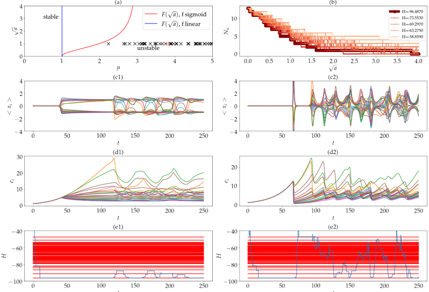
\n ## Charts/Graphs: Bifurcation Analysis and Dynamical System Behavior ### Overview The image presents a series of plots illustrating the bifurcation behavior of a dynamical system as a parameter (μ) is varied. It includes a bifurcation diagram, plots of the number of fixed points, time series of the average value of x, plots of the Lyapunov exponent, and plots of the entropy (H). The plots appear to be generated from numerical simulations. ### Components/Axes The image consists of six subplots labeled (a) through (f2). * **(a):** Bifurcation Diagram. X-axis: μ (ranging from approximately 0 to 5). Y-axis: `f(√n)` (ranging from approximately 0 to 4). Two curves are plotted: `F(√n)` (red, sigmoid) and `f(√n)` (black, linear). 'Stable' and 'Unstable' regions are indicated. 'x' marks are scattered along the black curve. * **(b):** Number of Fixed Points. X-axis: `√n` (ranging from approximately 0 to 4). Y-axis: `N` (number of fixed points, ranging from approximately 0 to 10). Multiple lines are plotted, each representing a different value of H (labeled in the legend). * **(c1):** Time Series of `<x>`. X-axis: t (time, ranging from approximately 0 to 250). Y-axis: `<x>` (average value of x, ranging from approximately -4 to 4). Multiple lines are plotted, each representing a different trajectory. * **(c2):** Time Series of `<x>`. X-axis: t (time, ranging from approximately 0 to 250). Y-axis: `<x>` (average value of x, ranging from approximately -4 to 4). Multiple lines are plotted, each representing a different trajectory. * **(d1):** Lyapunov Exponent. X-axis: t (time, ranging from approximately 0 to 250). Y-axis: `e₁` (Lyapunov exponent, ranging from approximately 0 to 20). Multiple lines are plotted, each representing a different trajectory. * **(d2):** Lyapunov Exponent. X-axis: t (time, ranging from approximately 0 to 250). Y-axis: `e₁` (Lyapunov exponent, ranging from approximately 0 to 20). Multiple lines are plotted, each representing a different trajectory. * **(e1):** Entropy (H). X-axis: t (time, ranging from approximately 0 to 250). Y-axis: H (entropy, ranging from approximately -100 to 0). The plot is filled with color, representing the entropy value. * **(e2):** Entropy (H). X-axis: t (time, ranging from approximately 0 to 250). Y-axis: H (entropy, ranging from approximately -100 to 0). The plot consists of vertical lines, each representing the entropy value at a given time. **Legend (b):** * H = -96.4870 (dark red) * H = -73.5530 (red) * H = -69.2760 (orange) * H = -63.2790 (yellow) * H = -56.8990 (light yellow) ### Detailed Analysis or Content Details * **(a):** The red sigmoid curve represents a stable state for low values of μ. As μ increases, the black linear curve shows instability, and 'x' marks indicate multiple fixed points. * **(b):** The number of fixed points (N) initially decreases with increasing `√n` for all H values. The lines then become relatively flat, indicating a stable number of fixed points. The dark red line (H = -96.4870) has the highest number of fixed points across the range. * **(c1):** The time series shows a relatively stable oscillation around `<x>` = 2 for the initial time period. After approximately t=100, the oscillations become more complex and varied. * **(c2):** The time series shows chaotic oscillations with a wide range of values for `<x>`. The oscillations appear to be aperiodic. * **(d1):** The Lyapunov exponent `e₁` is initially close to zero, indicating stability. As time progresses, `e₁` increases for some trajectories, suggesting a transition to chaos. * **(d2):** The Lyapunov exponent `e₁` shows a more pronounced positive value for many trajectories, confirming chaotic behavior. * **(e1):** The entropy (H) is initially low (red color) and then increases (towards yellow) as time progresses, indicating increasing complexity and disorder. * **(e2):** The entropy (H) fluctuates over time, with periods of high and low entropy. The vertical lines indicate discrete entropy values at each time step. ### Key Observations * The bifurcation diagram (a) suggests a transition from stable to unstable behavior as μ increases. * The number of fixed points (b) decreases with increasing `√n` and is influenced by the value of H. * The time series plots (c1 and c2) demonstrate a transition from stable oscillations to chaotic behavior. * The Lyapunov exponent plots (d1 and d2) confirm the presence of chaos, as indicated by positive values of `e₁`. * The entropy plots (e1 and e2) show an increase in complexity and disorder as the system evolves. ### Interpretation The data suggests a system undergoing a bifurcation from a stable state to a chaotic state as the parameter μ is increased. The bifurcation diagram (a) visually represents this transition. The number of fixed points (b) reflects the system's stability, with fewer fixed points indicating instability. The time series plots (c1 and c2) and Lyapunov exponent plots (d1 and d2) provide evidence of chaotic behavior, characterized by aperiodic oscillations and positive Lyapunov exponents. The entropy plots (e1 and e2) quantify the increasing complexity and disorder associated with chaos. The different values of H in plot (b) likely represent different initial conditions or parameter settings that influence the system's behavior. The plots collectively demonstrate a typical route to chaos, where a system initially exhibits stable behavior, then undergoes a bifurcation, and eventually settles into a chaotic state. The system is sensitive to initial conditions, as evidenced by the diverging trajectories in the time series and Lyapunov exponent plots.