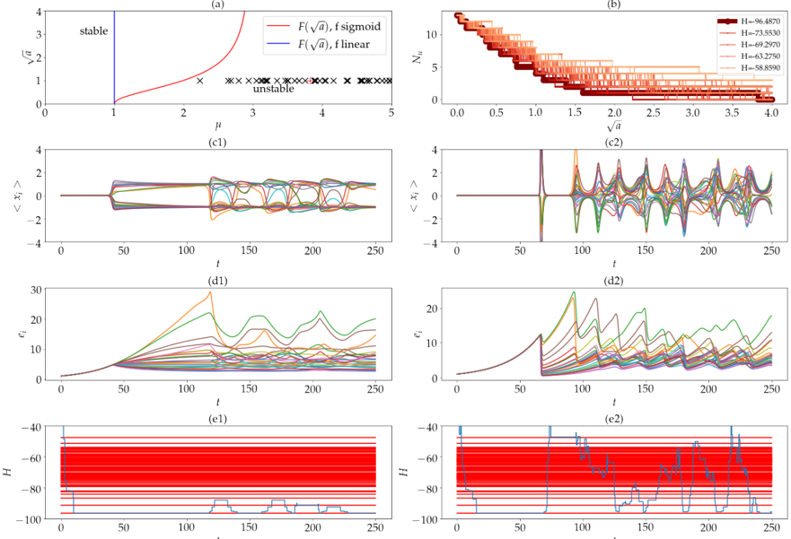
## Grid of Subplots: System Dynamics and Stability Analysis ### Overview The image contains six subplots (a)-(f) arranged in a 2x3 grid, depicting system dynamics, stability thresholds, and time-dependent behaviors. Each subplot includes labeled axes, legends, and data series. The visual elements suggest a focus on nonlinear dynamics, bifurcation analysis, and parameter sensitivity. --- ### Components/Axes #### Subplot (a): Stability Threshold - **X-axis**: μ (parameter, range: 0–5) - **Y-axis**: √a (square root of a parameter, range: 0–4) - **Legend**: - Red line: F(√a), fsigmoid - Blue line: F(√a), flinear - **Key elements**: - Vertical blue line at μ = 1 (labeled "stable") - Red line starts at (μ=1, √a=0) and curves upward - Blue line is horizontal at √a ≈ 0.5 - "Unstable" region marked with × symbols for μ > 1 #### Subplot (b): Parameter Space Heatmap - **X-axis**: √a (range: 0–4, increments of 0.5) - **Y-axis**: N_u (discrete values: 0–10) - **Z-axis**: H (values: 58.8590, 63.2750, 69.2970, 73.5530, 96.4870) - **Legend**: Color-coded H values (dark red to light orange) - **Key elements**: - Bars decrease in height as √a increases - H values correspond to specific √a increments #### Subplots (c1) and (c2): Time Series of <x_i> - **X-axis**: t (time, range: 0–250) - **Y-axis**: <x_i> (mean of x_i, range: -4–4) - **Legend**: Multiple colored lines (no explicit labels) - **Key elements**: - (c1): Lines oscillate around 0 with damping - (c2): Lines show sustained oscillations with varying amplitudes #### Subplots (d1) and (d2): Time Series of ε_i - **X-axis**: t (time, range: 0–250) - **Y-axis**: ε_i (error term, range: 0–30) - **Legend**: Multiple colored lines (no explicit labels) - **Key elements**: - (d1): Lines show sharp peaks and decay - (d2): Lines exhibit chaotic oscillations #### Subplots (e1) and (e2): Time Series of H - **X-axis**: t (time, range: 0–250) - **Y-axis**: H (range: -100–0) - **Legend**: - (e1): Red lines (stable H), blue lines (transient H) - (e2): Red lines (stable H), blue lines (dynamic H) - **Key elements**: - (e1): Red lines dominate, with minor blue fluctuations - (e2): Blue lines show significant variability --- ### Detailed Analysis #### Subplot (a) - **Trend**: The red line (fsigmoid) transitions from stable (μ < 1) to unstable (μ > 1) with a sigmoidal curve. The blue line (flinear) remains constant at √a ≈ 0.5. - **Data Points**: - Stable region: μ ∈ [0, 1] - Unstable region: μ ∈ [1, 5] - F(√a), fsigmoid: At μ = 1, √a = 0; at μ = 5, √a ≈ 3.5 - F(√a), flinear: Constant √a ≈ 0.5 across μ #### Subplot (b) - **Trend**: H decreases monotonically as √a increases. Each H value corresponds to a specific √a increment (e.g., H = 96.4870 at √a = 0, H = 58.8590 at √a = 4). - **Data Points**: - H = 96.4870 at √a = 0 - H = 73.5530 at √a = 0.5 - H = 69.2970 at √a = 1.0 - H = 63.2750 at √a = 1.5 - H = 58.8590 at √a = 2.0 #### Subplots (c1) and (c2) - **Trend**: - (c1): Lines converge to 0 with damping oscillations (stable system). - (c2): Lines exhibit sustained oscillations (unstable or chaotic system). - **Data Points**: - (c1): <x_i> oscillates between -2 and 2, with amplitude decreasing over time. - (c2): <x_i> oscillates between -4 and 4, with no damping. #### Subplots (d1) and (d2) - **Trend**: - (d1): ε_i peaks at ~30, then decays to 0. - (d2): ε_i shows chaotic behavior with peaks up to ~20. - **Data Points**: - (d1): ε_i ≈ 0 at t = 0, peaks at t ≈ 50, decays to 0 by t ≈ 150. - (d2): ε_i fluctuates between 0 and 20, with no clear trend. #### Subplots (e1) and (e2) - **Trend**: - (e1): H remains near -60 to -80, with minor blue fluctuations. - (e2): H fluctuates between -60 and -100, with blue lines showing more variability. - **Data Points**: - (e1): H ≈ -60 (red), with small blue spikes at t ≈ 50, 100, 150. - (e2): H ≈ -60 (red), with blue lines dipping to -100 at t ≈ 50, 150. --- ### Key Observations 1. **Stability Threshold**: The vertical line at μ = 1 in (a) defines a critical bifurcation point. The system transitions from stable (μ < 1) to unstable (μ > 1). 2. **Parameter Sensitivity**: H decreases with increasing √a (subplot b), suggesting a trade-off between system complexity and stability. 3. **Time Dynamics**: - (c1) and (d1) show damped oscillations, indicating a stable system. - (c2) and (d2) exhibit sustained or chaotic oscillations, suggesting instability. 4. **H Variability**: Subplots (e1) and (e2) highlight how H evolves over time, with blue lines (possibly transient states) showing more variability than red lines (stable states). --- ### Interpretation - **Stability and Bifurcation**: The sigmoidal curve in (a) implies a nonlinear threshold for stability. The linear approximation (blue line) underestimates the system's response, highlighting the importance of nonlinear dynamics. - **Parameter Space**: The heatmap in (b) reveals that higher √a values correspond to lower H, possibly indicating reduced system efficiency or increased complexity. - **Time Series Behavior**: The oscillations in (c) and (d) suggest that the system's response depends on initial conditions or parameter choices. The damping in (c1) and (d1) contrasts with the chaos in (c2) and (d2), emphasizing the role of parameters in determining long-term behavior. - **H Dynamics**: The red lines in (e1) and (e2) represent stable states, while blue lines (transient or dynamic states) show greater variability, indicating sensitivity to perturbations. This analysis underscores the interplay between parameters (μ, √a, H) and system behavior, with critical thresholds and nonlinear dynamics shaping stability and oscillations.