## Chart: Density Plot of Female and Male Distributions
### Overview
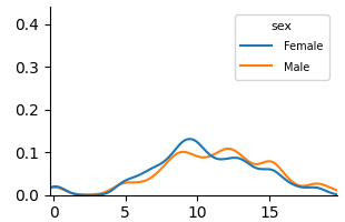
The image is a density plot comparing the distributions of two groups, "Female" and "Male". The plot shows the probability density of each group across a range of values on the x-axis.
### Components/Axes
* **X-axis:** The x-axis is unlabeled but ranges from approximately 0 to 20.
* **Y-axis:** The y-axis represents density, ranging from 0.0 to 0.4.
* **Legend:** Located in the top-right corner, the legend identifies the two data series:
* Blue line: "Female"
* Orange line: "Male"
### Detailed Analysis
* **Female (Blue Line):**
* The density starts near 0 at x=0.
* It gradually increases to approximately 0.06 around x=5.
* It peaks at around 0.13 near x=10.
* It decreases to approximately 0.08 around x=13.
* It fluctuates around 0.08-0.10 between x=13 and x=16.
* It decreases to near 0 at x=20.
* **Male (Orange Line):**
* The density starts near 0 at x=0.
* It gradually increases to approximately 0.04 around x=5.
* It increases to approximately 0.10 around x=9.
* It peaks at around 0.11 near x=13.
* It decreases to approximately 0.02 around x=18.
* It decreases to near 0 at x=20.
### Key Observations
* Both distributions start near 0 and end near 0.
* The "Female" distribution has a higher peak density (approximately 0.13) compared to the "Male" distribution (approximately 0.11).
* The "Female" distribution peaks earlier (around x=10) than the "Male" distribution (around x=13).
* The "Male" distribution has a broader peak, while the "Female" distribution has a sharper peak.
### Interpretation
The density plot compares the distributions of "Female" and "Male" groups across an unlabeled x-axis. The "Female" group shows a higher density peak at an earlier value, suggesting a higher concentration of data points around x=10. The "Male" group has a broader peak, indicating a more dispersed distribution. Without knowing what the x-axis represents, it's difficult to provide a more specific interpretation. However, the plot suggests that there are notable differences in the distributions of the two groups.