## Diagram: Piecewise Linear Function
### Overview
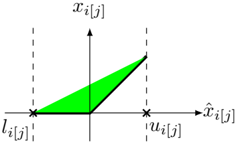
The image depicts a piecewise linear function, shaded in green, defined over an interval. The function is zero up to a lower bound, then increases linearly to an upper bound. The x-axis is labeled as `x̂_i[j]` and the y-axis is labeled as `x_i[j]`. The lower and upper bounds are marked as `l_i[j]` and `u_i[j]` respectively.
### Components/Axes
* **x-axis:** `x̂_i[j]`
* Lower bound marker: `l_i[j]`
* Upper bound marker: `u_i[j]`
* **y-axis:** `x_i[j]`
* **Function:** Piecewise linear, shaded in green.
* **Vertical dashed lines:** Indicate the lower and upper bounds on the x-axis.
### Detailed Analysis
The function is defined as follows:
* For `x̂_i[j] < l_i[j]`, the function value `x_i[j]` is 0.
* For `l_i[j] <= x̂_i[j] <= u_i[j]`, the function increases linearly from 0 to a positive value.
* For `x̂_i[j] > u_i[j]`, the function continues to increase linearly.
The x-axis ranges from approximately -1 to 1, with `l_i[j]` at approximately -0.75 and `u_i[j]` at approximately 0.75. The y-axis ranges from 0 to approximately 1.
### Key Observations
* The function is zero for values of `x̂_i[j]` less than `l_i[j]`.
* The function increases linearly between `l_i[j]` and `u_i[j]`.
* The function continues to increase linearly beyond `u_i[j]`.
### Interpretation
The diagram illustrates a piecewise linear function that could represent a thresholding or activation function. The function is zero until a certain threshold (`l_i[j]`) is reached, after which it increases linearly. This type of function is commonly used in machine learning and signal processing to introduce non-linearity into a system. The bounds `l_i[j]` and `u_i[j]` define the region where the linear increase occurs.