## Diagram: Bounded Linear Relationship with Feasible Region
### Overview
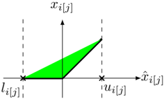
The image is a technical mathematical diagram illustrating a linear relationship between two variables, $\hat{x}_{i[j]}$ (estimated or predicted value) and $x_{i[j]}$ (actual or true value), within defined lower and upper bounds. A shaded green triangular region represents the set of all possible pairs $(\hat{x}_{i[j]}, x_{i[j]})$ that satisfy the constraints shown.
### Components/Axes
* **Horizontal Axis (x-axis):** Labeled $\hat{x}_{i[j]}$. This represents the estimated or predicted value.
* **Vertical Axis (y-axis):** Labeled $x_{i[j]}$. This represents the actual or true value.
* **Origin:** The axes intersect at the origin (0,0), which is a vertex of the shaded region.
* **Lower Bound Marker:** A point labeled $l_{i[j]}$ is marked on the horizontal axis to the left of the origin. A vertical dashed line extends upward from this point.
* **Upper Bound Marker:** A point labeled $u_{i[j]}$ is marked on the horizontal axis to the right of the origin. A vertical dashed line extends upward from this point.
* **Shaded Region:** A green-filled triangular area. Its vertices are:
1. The origin (0,0).
2. The point where the vertical line from $l_{i[j]}$ intersects a line from the origin. This point is in the second quadrant (negative $\hat{x}_{i[j]}$, positive $x_{i[j]}$).
3. The point where the vertical line from $u_{i[j]}$ intersects a line from the origin. This point is in the first quadrant (positive $\hat{x}_{i[j]}$, positive $x_{i[j]}$).
* **Boundary Lines:** The upper boundary of the green triangle is a straight line passing through the origin and the two intersection points described above. The lower boundary is the horizontal axis itself (where $x_{i[j]} = 0$) between $l_{i[j]}$ and $u_{i[j]}$.
### Detailed Analysis
* **Spatial Layout:** The legend/labels are placed directly on the axes and points. $l_{i[j]}$ is positioned at the bottom-left, $u_{i[j]}$ at the bottom-right, $\hat{x}_{i[j]}$ at the far right of the horizontal axis, and $x_{i[j]}$ at the top of the vertical axis.
* **Geometric Relationship:** The diagram defines a **cone** or **wedge** of feasible $(\hat{x}_{i[j]}, x_{i[j]})$ pairs. For any estimated value $\hat{x}_{i[j]}$ between $l_{i[j]}$ and $u_{i[j]}$, the corresponding actual value $x_{i[j]}$ is constrained to be non-negative and lies on or below the upper boundary line.
* **Trend/Flow:** The upper boundary line has a positive slope, indicating a direct, proportional relationship between $\hat{x}_{i[j]}$ and $x_{i[j]}$ at the limit of the feasible region. As $\hat{x}_{i[j]}$ increases from $l_{i[j]}$ to $u_{i[j]}$, the maximum possible value of $x_{i[j]}$ increases linearly.
* **Data Points:** No discrete data points are plotted. The diagram illustrates a continuous constraint region.
### Key Observations
1. **Asymmetry:** The feasible region is asymmetric around the vertical axis. The cone extends further into the positive $\hat{x}_{i[j]}$ domain (to $u_{i[j]}$) than into the negative domain (to $l_{i[j]}$), assuming $|u_{i[j]}| > |l_{i[j]}|$.
2. **Non-Negativity Constraint:** The shaded region lies entirely above the horizontal axis, imposing the constraint $x_{i[j]} \geq 0$.
3. **Bound-Dependent Range:** The range of possible $x_{i[j]}$ values is directly determined by the value of $\hat{x}_{i[j]}$ and the slope of the upper boundary. The bounds $l_{i[j]}$ and $u_{i[j]}$ define the domain of $\hat{x}_{i[j]}$ for which this relationship is visualized.
### Interpretation
This diagram is a **geometric representation of a constrained linear model or error bound**. It is commonly found in fields like optimization, control theory, or statistical estimation.
* **What it represents:** It likely depicts the relationship between a predicted/estimated variable ($\hat{x}_{i[j]}$) and the actual variable ($x_{i[j]}$), where the actual value is constrained to be non-negative and is bounded by a linear function of the estimate. The green area is the set of all physically or mathematically plausible pairs.
* **Relationship between elements:** The bounds $l_{i[j]}$ and $u_{i[j]}$ define the operational range of the estimator. The upper boundary line represents a **worst-case** or **limiting** relationship (e.g., maximum possible actual value for a given estimate). The lower boundary (the axis) represents the absolute minimum (zero).
* **Potential Context:** This could illustrate:
* The feasible set for a variable in a linear programming problem.
* The confidence region or error bounds for a linear estimator.
* A saturation or clipping function where the output ($x_{i[j]}$) is a scaled version of the input ($\hat{x}_{i[j]}$) but cannot be negative.
* **Notable Implication:** The diagram emphasizes that the relationship is not one-to-one. For a single estimate $\hat{x}_{i[j]}$, there is a range of possible actual values $x_{i[j]}$, bounded below by 0 and above by the linear function. The uncertainty or allowable error grows linearly with the magnitude of $\hat{x}_{i[j]}$.