## Autocorrelation Function (ACF) Plots for Different States
### Overview
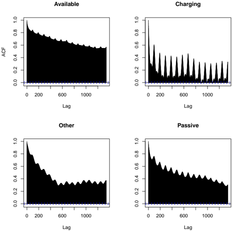
The image presents four Autocorrelation Function (ACF) plots, each representing a different state: Available, Charging, Other, and Passive. Each plot shows the correlation of a time series with its own past values as a function of the lag. The x-axis represents the lag, and the y-axis represents the autocorrelation coefficient (ACF).
### Components/Axes
* **Titles:**
* Top-left: Available
* Top-right: Charging
* Bottom-left: Other
* Bottom-right: Passive
* **X-axis (Lag):**
* Label: Lag
* Scale: 0 to 1000, with tick marks at 0, 200, 600, and 1000.
* **Y-axis (ACF):**
* Label: ACF
* Scale: 0.0 to 1.0, with tick marks at 0.0, 0.2, 0.4, 0.6, 0.8, and 1.0.
* **Dashed Blue Line:** A horizontal dashed blue line is present at y = 0.0 on each plot, indicating the threshold for statistical significance.
### Detailed Analysis
**1. Available:**
* **Trend:** The ACF starts at 1.0 and gradually decreases as the lag increases. The decay is relatively smooth, indicating a strong positive autocorrelation at short lags.
* **Values:**
* ACF at Lag 0: 1.0
* ACF at Lag 200: ~0.75
* ACF at Lag 600: ~0.6
* ACF at Lag 1000: ~0.5
**2. Charging:**
* **Trend:** The ACF exhibits a periodic pattern with peaks and troughs. The initial peak is at 1.0, followed by decreasing peaks and troughs as the lag increases.
* **Values:**
* ACF at Lag 0: 1.0
* ACF at Lag 100 (first trough): ~0.0
* ACF at Lag 200 (first peak): ~0.6
* ACF at Lag 300 (second trough): ~0.0
* ACF at Lag 400 (second peak): ~0.4
* ACF at Lag 1000: Peaks are around ~0.2, troughs are around ~0.0
**3. Other:**
* **Trend:** The ACF starts at 1.0 and decreases with oscillations as the lag increases.
* **Values:**
* ACF at Lag 0: 1.0
* ACF at Lag 200: ~0.6
* ACF at Lag 400: ~0.3
* ACF at Lag 600: ~0.4
* ACF at Lag 800: ~0.3
* ACF at Lag 1000: ~0.3
**4. Passive:**
* **Trend:** The ACF starts at 1.0 and decreases as the lag increases, with some oscillations.
* **Values:**
* ACF at Lag 0: 1.0
* ACF at Lag 200: ~0.7
* ACF at Lag 400: ~0.5
* ACF at Lag 600: ~0.4
* ACF at Lag 800: ~0.3
* ACF at Lag 1000: ~0.2
### Key Observations
* The "Available" state shows a smooth decay in autocorrelation, indicating a persistent positive correlation over time.
* The "Charging" state exhibits a strong periodic pattern, suggesting a cyclical behavior in the charging process.
* The "Other" and "Passive" states show decaying autocorrelation with oscillations, indicating some degree of short-term correlation.
### Interpretation
The ACF plots provide insights into the temporal dependencies within each state. The "Available" state suggests that if the system is available at one point in time, it is likely to remain available for a considerable period. The "Charging" state's periodic pattern indicates a regular charging cycle. The "Other" and "Passive" states show more complex autocorrelation structures, suggesting a mix of short-term dependencies and random fluctuations. These plots can be used to model and predict the behavior of the system in each state.