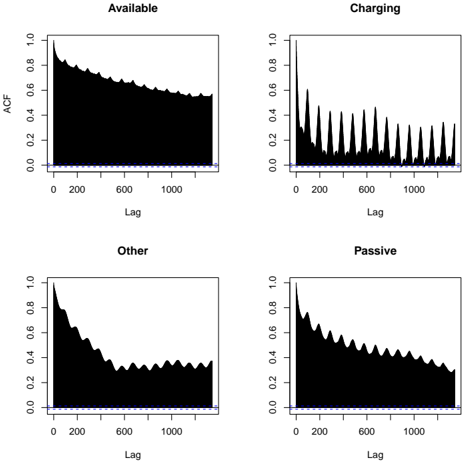
## Line Chart: Autocorrelation Function (ACF) Across Lag for Different States ### Overview The image displays four subplots arranged in a 2x2 grid, each representing the Autocorrelation Function (ACF) across lag values (0–1000) for distinct states: **Available**, **Charging**, **Other**, and **Passive**. All subplots share identical axes (Lag on x-axis, ACF on y-axis) and a horizontal dotted line at ACF = 0.02. The shaded black areas represent the magnitude of ACF values, with varying patterns across states. --- ### Components/Axes - **X-axis (Lag)**: Ranges from 0 to 1000, labeled "Lag". Incremental markers are present but unlabeled. - **Y-axis (ACF)**: Ranges from 0.0 to 1.0, labeled "ACF". Markers at 0.0, 0.2, 0.4, 0.6, 0.8, 1.0. - **Dotted Line**: Horizontal line at ACF = 0.02, spanning all subplots. - **Shaded Areas**: Black regions below the dotted line indicate ACF values. No explicit legend, but subplot titles act as categorical labels. --- ### Detailed Analysis #### **Available** - **Trend**: Gradual decline in ACF from ~0.8 at lag 0 to ~0.4 at lag 1000. - **Key Feature**: Smooth, consistent decay without spikes. #### **Charging** - **Trend**: Sharp, periodic spikes (e.g., ~0.8 at lags 200, 400, 600, 800, 1000) with decreasing amplitude. - **Key Feature**: Regular oscillations, suggesting cyclical behavior. #### **Other** - **Trend**: Erratic fluctuations with no clear pattern. ACF starts at ~0.8, dips to ~0.2 at lag 400, then rises to ~0.6 at lag 800 before stabilizing. - **Key Feature**: High variability, potential noise or irregularity. #### **Passive** - **Trend**: Steady decline from ~0.8 at lag 0 to ~0.3 at lag 1000, with minor oscillations. - **Key Feature**: Smoother decay than "Available", with slight undulations. --- ### Key Observations 1. **Threshold Significance**: The dotted line at ACF = 0.02 likely represents a statistical cutoff (e.g., 95% confidence interval). All shaded areas remain above this threshold, indicating persistent correlation across lags. 2. **State-Specific Patterns**: - **Charging** exhibits the most structured behavior (periodic spikes). - **Other** shows the least predictability (noise-like fluctuations). 3. **Decay Rates**: "Available" and "Passive" demonstrate gradual decay, while "Charging" maintains periodic relevance. --- ### Interpretation - **ACF Decay**: The gradual decline in "Available" and "Passive" suggests diminishing correlation over time, typical for stationary processes. The sharper decay in "Passive" may indicate faster mean reversion. - **Charging Spikes**: Regular peaks imply recurring events or interventions (e.g., scheduled maintenance, cyclical demand). The decreasing amplitude suggests diminishing impact over time. - **Other State**: High variability could reflect external noise, unmodeled factors, or transient states. Further investigation is warranted to identify drivers. - **Threshold Relevance**: All states maintain ACF > 0.02, implying correlations remain statistically significant even at high lags. This may indicate long-memory processes or persistent dependencies. --- ### Component Isolation - **Header**: Subplot titles ("Available", "Charging", etc.) are positioned at the top of each plot. - **Main Chart**: Shaded areas dominate, with the dotted line providing a reference. - **Footer**: No additional annotations or labels beyond axes. --- ### Conclusion The ACF patterns reveal distinct temporal dependencies across states. "Charging" suggests cyclical interventions, while "Other" highlights unpredictability. The consistent threshold above 0.02 underscores persistent correlations, warranting further analysis of underlying mechanisms.