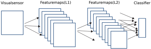
## Diagram: Neural Network Architecture for Image Classification ### Overview The diagram illustrates a simplified neural network architecture for image classification. It depicts the flow of data from a visual sensor through two feature map layers (L1 and L2) to a classifier. The structure uses rectangular blocks to represent computational layers and arrows to indicate data flow. ### Components/Axes - **Visual Sensor**: Input layer (leftmost block). - **Featuremaps(L1)**: First layer of feature extraction (middle section with multiple stacked blocks). - **Featuremaps(L2)**: Second layer of feature extraction (middle section with multiple stacked blocks). - **Classifier**: Output layer (rightmost block). - **Arrows**: Represent data flow between layers. ### Detailed Analysis - **Visual Sensor**: Positioned at the far left, serving as the input source for raw image data. - **Featuremaps(L1)**: Composed of 8 stacked blocks, indicating multiple feature maps extracted at this layer. Arrows show data transformation from the sensor to L1. - **Featuremaps(L2)**: Contains 6 stacked blocks, suggesting reduced dimensionality or increased abstraction compared to L1. Arrows indicate further processing from L1 to L2. - **Classifier**: Single block on the far right, receiving aggregated features from L2 for final classification. - **Flow Direction**: Left-to-right progression, typical of feedforward neural networks. ### Key Observations - **Layer Complexity**: L1 has more feature maps (8) than L2 (6), possibly indicating downsampling or hierarchical feature abstraction. - **No Explicit Activation Functions**: The diagram omits details like activation functions (e.g., ReLU, sigmoid), focusing only on structural flow. - **Simplified Representation**: Blocks are uniform in size, but real-world implementations often vary block dimensions based on layer depth. ### Interpretation This architecture represents a convolutional neural network (CNN) simplified for clarity. The visual sensor captures raw pixel data, which is processed through two convolutional layers (L1 and L2) to extract hierarchical features. The classifier then uses these features to make predictions. The reduction in feature maps from L1 to L2 suggests spatial downsampling, a common technique to reduce computational load while retaining critical information. The absence of explicit activation functions or pooling layers implies this is a high-level conceptual diagram rather than a detailed implementation blueprint. The flow emphasizes the end-to-end pipeline from input to output, critical for understanding how raw images are transformed into class probabilities.