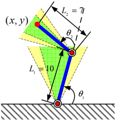
## Kinematic Diagram: 2-Link Planar Robotic Arm ### Overview This image is a technical schematic representing a two-dimensional (planar) robotic manipulator with two revolute joints (an RR linkage). It illustrates the geometric and kinematic parameters required to calculate the position of the end effector, including link lengths, joint angles, and angular constraints (joint limits). ### Components and Variables The diagram is composed of several distinct visual and textual elements, spatially arranged as follows: * **Ground/Base:** Located at the bottom, represented by a horizontal black line with diagonal gray hatching beneath it, indicating a fixed, immovable surface. * **Joints (Nodes):** Three distinct points of articulation/termination: * **Base Joint:** Bottom-center, resting on the ground line. Depicted as a red circle with a white center and black outline. * **Elbow Joint:** Center-right. Depicted identically to the base joint. * **End Effector:** Top-left. Depicted as a solid red circle. * **Links (Arms):** Two thick blue line segments connecting the joints. * **Text Labels & Values:** * **$(x, y)$**: Located at the top-left, adjacent to the end effector. * **$L_1 = 10$**: Located in the lower-left quadrant, positioned next to a dimension line parallel to the first link. * **$L_2 = 7$**: Located in the upper-right quadrant, positioned next to a dimension line parallel to the second link. * **$\theta_1$**: Located at the bottom-right, labeling an angular arc. * **$\theta_2$**: Located near the center-right (above the elbow joint), labeling an angular arc. * **Constraint Zones (Shaded Areas):** Cone-shaped sectors originating from the base and elbow joints, featuring a green inner area with a grid pattern and yellow outer edges bounded by dashed lines. ### Content Details **1. Base and Link 1 ($L_1$)** * **Positioning:** Originates at the Base Joint on the ground. The thick blue line extends upwards and slightly to the right. * **Length:** A dimension line with arrows at both ends runs parallel to this link. The text explicitly states **$L_1 = 10$**. * **Angle ($\theta_1$):** An arc with an arrowhead originates from the right-side horizontal ground line and curves counter-clockwise to meet Link 1. This denotes the absolute base angle, labeled **$\theta_1$**. Visually, this angle is approximately $75^\circ$ to $80^\circ$. * **Constraints:** A shaded sector originates from the base joint. The central portion of the sector is green with a grid, flanked by solid yellow regions. Dashed lines mark the absolute outer boundaries of the yellow regions. This visually represents the allowable range of motion for $\theta_1$. **2. Elbow and Link 2 ($L_2$)** * **Positioning:** Originates at the Elbow Joint (connecting $L_1$ and $L_2$). The thick blue line extends upwards and to the left. * **Reference Line:** A dashed black line extends straight out from the Elbow Joint, continuing the exact trajectory/vector of Link 1. * **Length:** A dimension line with arrows at both ends runs parallel to this second link. The text explicitly states **$L_2 = 7$**. * **Angle ($\theta_2$):** An arc with an arrowhead originates from the dashed reference line and curves counter-clockwise to meet Link 2. This denotes the relative joint angle, labeled **$\theta_2$**. Visually, this angle is obtuse, approximately $135^\circ$ to $150^\circ$. * **Constraints:** Similar to Link 1, a shaded sector (green grid center, yellow edges, dashed boundaries) originates from the Elbow Joint, representing the allowable range of motion for $\theta_2$ relative to Link 1. **3. End Effector** * **Positioning:** The terminal end of Link 2. * **Coordinates:** Labeled explicitly as **$(x, y)$**, representing the Cartesian coordinates of the robot's tip in 2D space. ### Key Observations * **Relative vs. Absolute Angles:** The diagram clearly distinguishes between an absolute angle ($\theta_1$ is measured from the fixed ground) and a relative angle ($\theta_2$ is measured from the extended axis of the previous link). This is standard Denavit-Hartenberg convention for robotic kinematics. * **Visualizing Limits:** The green and yellow shaded regions are critical. They do not represent physical objects, but rather the mathematical/mechanical limits of the joints. The green area likely represents the normal/safe operating range, while the yellow areas represent warning zones approaching the mechanical hard-stops (dashed lines). * **Proportions:** The visual lengths of the blue lines roughly correspond to their stated values ($L_1=10$ is visibly longer than $L_2=7$). ### Interpretation This diagram is a classic representation of a **Forward Kinematics** problem in robotics. Forward kinematics involves calculating the position of the end effector $(x, y)$ given the link lengths ($L_1, L_2$) and the joint angles ($\theta_1, \theta_2$). Based on the geometric relationships explicitly detailed in the image, the mathematical equations governing this system are implied: * $x = L_1 \cos(\theta_1) + L_2 \cos(\theta_1 + \theta_2)$ * $y = L_1 \sin(\theta_1) + L_2 \sin(\theta_1 + \theta_2)$ **Reading between the lines (Peircean investigative):** The inclusion of the green and yellow constraint zones elevates this from a simple geometry problem to a practical robotics engineering diagram. In real-world applications, joints cannot rotate infinitely due to internal wiring, motors, or physical casing. * If an engineer were writing a path-planning algorithm for this arm, they would use the dashed lines as absolute constraints (e.g., $\theta_{1_{min}} \le \theta_1 \le \theta_{1_{max}}$). * The transition from green to yellow suggests a control system where moving into the yellow zone might trigger a software speed reduction to prevent mechanical damage upon hitting the dashed-line limit. * Furthermore, knowing these limits is essential for **Inverse Kinematics** (calculating required angles to reach a specific $(x,y)$ point), as some points in space might be mathematically reachable but physically impossible due to the joint limits shown by the shaded cones.