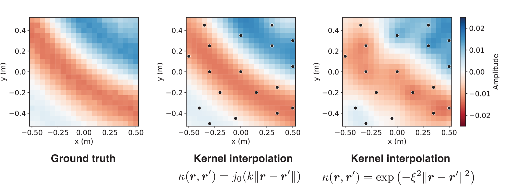
\n ## Heatmaps: Kernel Interpolation Comparison ### Overview The image presents three heatmaps side-by-side, comparing a "Ground truth" to two different "Kernel interpolation" methods. Each heatmap visualizes a two-dimensional distribution of "Amplitude" over a spatial area defined by x and y coordinates. The interpolation methods are differentiated by their kernel functions, displayed as equations below the respective heatmaps. Black dots are overlaid on the Kernel Interpolation heatmaps, presumably representing sample points. ### Components/Axes Each heatmap shares the following components: * **X-axis:** Labeled "x (m)", ranging from approximately -0.50 to 0.50 meters. * **Y-axis:** Labeled "y (m)", ranging from approximately -0.40 to 0.40 meters. * **Color Scale:** A vertical color bar on the right side represents "Amplitude", ranging from -0.02 to 0.02. The color gradient transitions from blue (negative amplitude) through white (zero amplitude) to red (positive amplitude). * **Titles:** Each heatmap has a title indicating its content: "Ground truth", "Kernel interpolation" (with the first kernel equation), and "Kernel interpolation" (with the second kernel equation). * **Kernel Equations:** Below the "Kernel interpolation" heatmaps are equations defining the kernel functions used: * κ(r, r') = j₀(k||r - r'||) * κ(r, r') = exp(-ξ²||r - r'||²) ### Detailed Analysis or Content Details **1. Ground Truth Heatmap:** * The heatmap displays a roughly elliptical pattern. * The highest amplitude (red) is centered around x = 0.0 m and y = 0.0 m. * Amplitude decreases radially from the center, transitioning through white to blue. * The maximum positive amplitude appears to be around +0.015. * The maximum negative amplitude appears to be around -0.015. **2. Kernel Interpolation (j₀(k||r - r'||)) Heatmap:** * This heatmap shows a similar elliptical pattern to the "Ground truth", but with more pronounced discrete features. * Six black dots are overlaid on the heatmap. Their approximate coordinates are: * (-0.25, -0.25) * (-0.25, 0.25) * (0.0, -0.25) * (0.0, 0.25) * (0.25, -0.25) * (0.25, 0.25) * The amplitude values at the dot locations appear to be positive, with the color ranging from light blue to red. * The maximum positive amplitude appears to be around +0.02. * The maximum negative amplitude appears to be around -0.01. **3. Kernel Interpolation (exp(-ξ²||r - r'||²)) Heatmap:** * This heatmap also displays an elliptical pattern, but it appears smoother than the previous interpolation. * Six black dots are overlaid on the heatmap, at the same approximate coordinates as the previous heatmap. * The amplitude values at the dot locations appear to be positive, with the color ranging from light blue to red. * The maximum positive amplitude appears to be around +0.018. * The maximum negative amplitude appears to be around -0.01. ### Key Observations * Both kernel interpolation methods attempt to reconstruct the "Ground truth" distribution. * The first kernel interpolation (j₀) produces a more discrete, less smooth result, with sharper transitions in amplitude. * The second kernel interpolation (exp) produces a smoother, more continuous result. * The black dots in the interpolation heatmaps likely represent the data points used for interpolation. * The amplitude scale is slightly different between the "Ground truth" and the interpolation heatmaps, with the interpolation methods reaching slightly higher positive amplitudes. ### Interpretation The image demonstrates a comparison of different kernel interpolation methods for reconstructing a two-dimensional field from a set of discrete sample points. The "Ground truth" represents the original, continuous field. The two kernel interpolation methods aim to approximate this field based on the sampled data (represented by the black dots). The choice of kernel function significantly impacts the quality of the interpolation. The Bessel function (j₀) results in a more localized interpolation, potentially capturing finer details but also introducing artifacts. The exponential function (exp) provides a smoother interpolation, potentially sacrificing some detail but reducing artifacts. The slight differences in the amplitude scale suggest that the interpolation methods may introduce some bias or scaling effects. The overall goal is to find an interpolation method that accurately reconstructs the "Ground truth" field with minimal error and artifacts. The visual comparison suggests that the exponential kernel provides a more visually appealing and potentially more accurate reconstruction in this case, but a quantitative analysis would be needed to confirm this.