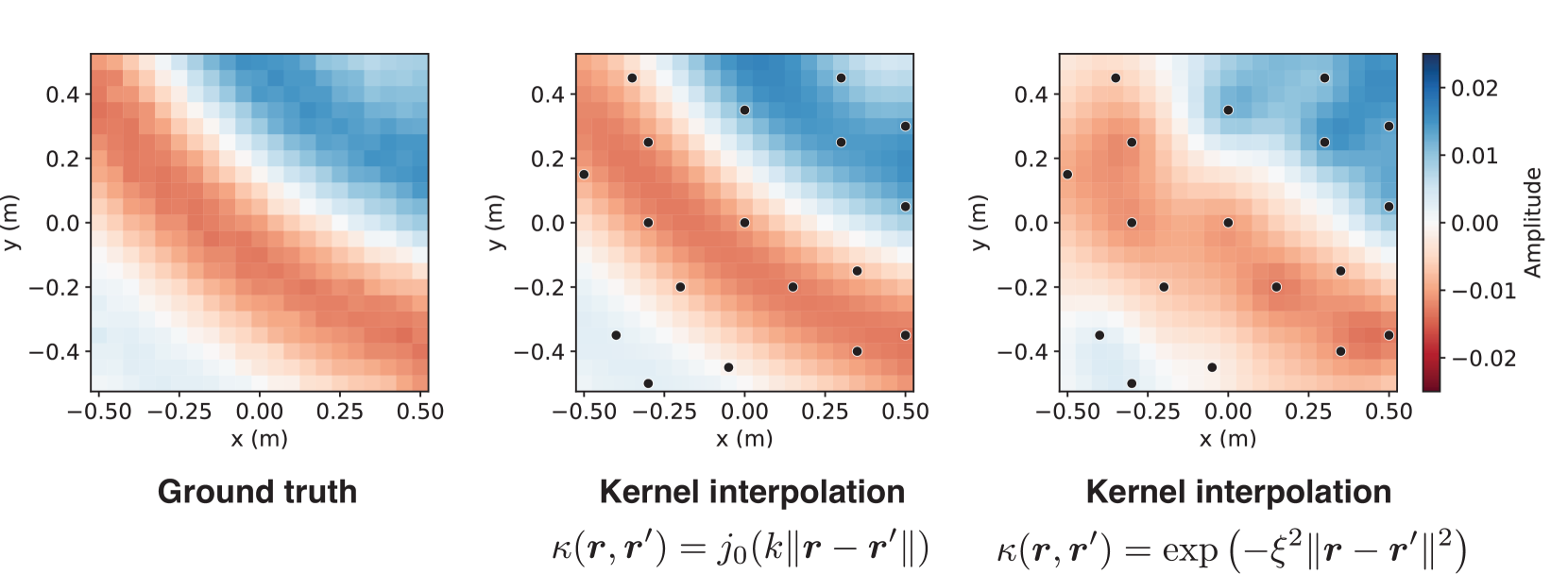
## Heatmap Visualization: Kernel Interpolation Comparison ### Overview The image presents three side-by-side panels comparing spatial amplitude distributions. The left panel shows a "Ground truth" reference, while the right two panels demonstrate kernel interpolation methods using different basis functions. All panels share identical spatial coordinates (-0.5 to 0.5 meters on both axes) and amplitude scales (-0.02 to 0.02). ### Components/Axes - **X-axis**: Spatial coordinate (x) in meters, ranging from -0.5 to 0.5 - **Y-axis**: Spatial coordinate (y) in meters, ranging from -0.5 to 0.5 - **Color Scale**: Amplitude values from -0.02 (dark red) to 0.02 (dark blue) - **Legend**: Single colorbar on the right panel indicating amplitude magnitude - **Text Elements**: - Panel titles: "Ground truth", "Kernel interpolation", "Kernel interpolation" - Kernel function definitions: - Left kernel: $ \kappa(\mathbf{r}, \mathbf{r}') = j_0(k\|\mathbf{r} - \mathbf{r}'\|) $ - Right kernel: $ \kappa(\mathbf{r}, \mathbf{r}') = \exp(-\xi^2\|\mathbf{r} - \mathbf{r}'\|^2) $ ### Detailed Analysis 1. **Ground Truth Panel**: - Smooth linear gradient from dark red (negative amplitude) in bottom-left to dark blue (positive amplitude) in top-right - No discrete data points present - Amplitude transition occurs diagonally across the plot 2. **Left Kernel Interpolation (Bessel Function)**: - Similar gradient pattern to ground truth but with 15 black data points overlaid - Points distributed across all quadrants with higher concentration near: - (-0.4, 0.3) - (0.1, -0.2) - (0.3, 0.4) - Color transitions show slight smoothing artifacts near data points 3. **Right Kernel Interpolation (Gaussian Function)**: - Similar gradient pattern with 18 black data points - Points show stronger clustering in: - Top-right quadrant (0.2-0.5 x, 0.2-0.4 y) - Bottom-left quadrant (-0.3-0.0 x, -0.4-0.0 y) - Color transitions appear more diffused compared to ground truth ### Key Observations 1. Both kernel methods preserve the general gradient direction of the ground truth 2. Bessel function interpolation maintains sharper amplitude transitions 3. Gaussian kernel introduces more amplitude smoothing, particularly noticeable in: - Reduced contrast near (0.0, 0.0) - Blurred transition between positive/negative regions 4. Data point distribution differs between kernels: - Bessel: More uniform spatial distribution - Gaussian: Clustered in specific regions ### Interpretation The visualization demonstrates how different kernel functions affect spatial interpolation: - The Bessel function kernel ($j_0$) preserves amplitude variations more faithfully to the ground truth, particularly in maintaining the diagonal amplitude transition - The Gaussian kernel introduces artificial smoothing, especially noticeable in the central region where amplitude should transition most sharply - Data point placement suggests the Bessel kernel better captures localized amplitude features, while the Gaussian kernel tends to average values across larger spatial regions - The amplitude scale consistency across panels confirms both methods operate within the same dynamic range as the ground truth The differences highlight the trade-off between interpolation accuracy and smoothing effects in kernel-based methods, with the Bessel function providing closer approximation to the ground truth at the cost of potential overfitting to discrete data points.