## Diagram: Transformer Model Training and Inference
### Overview
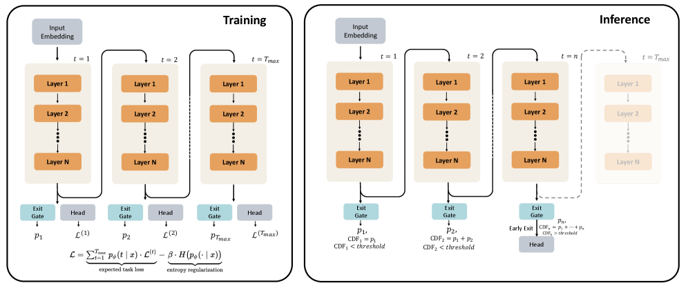
The image presents a diagram illustrating the training and inference processes of a transformer model. It depicts the flow of data through multiple layers over time steps, highlighting the differences in how the model operates during these two phases. The diagram focuses on the concept of "early exiting" during inference, where the model can potentially terminate processing at earlier layers based on a confidence threshold.
### Components/Axes
The diagram is divided into two main sections: "Training" (left) and "Inference" (right). Both sections share a similar structure, consisting of:
* **Input Embedding:** The initial stage where input data is converted into a vector representation.
* **Layer 1 to Layer N:** A series of stacked layers representing the transformer's core processing units. Each layer receives input from the previous layer.
* **Exit Gate:** A component that determines whether the processing should continue to the next layer or terminate.
* **Head:** The final output layer.
* **Time Steps (t):** Indicated as t=1, t=2, and t=Tmax.
* **Equation:** A loss function equation is present at the bottom of the "Training" section.
### Detailed Analysis or Content Details
**Training Section:**
* The "Training" section shows the data flowing sequentially through all N layers for each time step (t=1 to t=Tmax).
* Each layer outputs to an "Exit Gate" and a "Head". The outputs of the "Head" at each time step are denoted as L(1), L(2), and L(Tmax).
* The equation at the bottom reads: "L = Σt Ps(t x) - β H(Ps(t x))", with labels "expected task loss" and "entropy regularization".
**Inference Section:**
* The "Inference" section demonstrates the "early exit" mechanism.
* At each layer, the "Exit Gate" calculates a cumulative distribution function (CDF).
* The CDF is calculated as the sum of probabilities from previous layers (e.g., CDF1 = P1, CDF2 = P1 + P2).
* If the CDF exceeds a predefined "threshold", the processing terminates, and the "Head" receives the output from the current layer. This is indicated by the dashed arrow labeled "Early Exit".
* The CDF calculation is shown as: "CDF<sub>n</sub> = P<sub>1</sub> + ... + P<sub>n</sub>".
* The condition for early exit is "CDF<sub>n</sub> > threshold".
* The final layer (Layer N) at t=Tmax still outputs to the "Head" if early exit does not occur.
**Layer Details:**
* Each layer is represented by an orange rectangle labeled "Layer 1", "Layer 2", and "Layer N".
* The arrows indicate the flow of data from the "Input Embedding" through the layers and to the "Exit Gate" and "Head".
### Key Observations
* The diagram highlights the key difference between training and inference: during training, the model processes data through all layers at each time step, while during inference, it can potentially exit early based on confidence.
* The "early exit" mechanism is designed to improve inference speed and efficiency by reducing the computational cost for simpler inputs.
* The loss function equation suggests a combination of task loss and entropy regularization, which is common in transformer training to encourage diverse and informative representations.
* The CDF calculation and thresholding mechanism provide a probabilistic approach to determining when to terminate processing.
### Interpretation
The diagram illustrates a technique to optimize transformer models for faster inference. By allowing the model to exit early when it reaches a sufficient level of confidence, the computational cost can be significantly reduced, especially for inputs that do not require full processing. The use of a cumulative distribution function (CDF) and a threshold provides a principled way to make this decision. The training process, as indicated by the loss function, aims to learn representations that are both accurate and diverse, which is crucial for the effectiveness of the early exit mechanism. The entropy regularization term in the loss function likely encourages the model to explore different possible outputs, making it more robust and less prone to premature termination. The diagram suggests a trade-off between accuracy and efficiency, where early exiting can potentially lead to a slight decrease in accuracy but a significant improvement in speed. This is a common optimization strategy in real-world applications where latency is a critical factor.